Explanation
In this example, the goal is to list the 10 most frequently occurring text values in a range, in descending order by count, as seen in the range in E5:F14. This is an advanced formula that requires a number of nested functions. However, it is an excellent example of the power of dynamic array formulas in Excel . For convenience, data is the named range B5:B104. This range contains 100 random color names.
Get unique values
The first step in this problem is to get a list of unique colors from the data. This is easy to do with the UNIQUE function :
UNIQUE(data) // get unique colors
Since there 23 unique colors in B5:B104, UNIQUE returns an array containing 23 color names:
{"Violet";"Maroon";"Blue";"Pink";"Lime";"Navy";"Yellow";"White";"Cyan";"Teal";"Gold";"Orange";"Peach";"Black";"Turquoise";"Tan";"Red";"Green";"Gray";"Indigo";"Brown";"Purple";"Silver"}
Count unique values
Now that we have a list of values, the next step is to get a count for each unique value. This can be done with the COUNTIF function like this:
=COUNTIF(data,UNIQUE(data))
Here, the UNIQUE function returns the unique values in the data as the criteria argument, and COUNTIF calculates a count for each value. The result is an array with 23 counts like this:
{11;5;4;9;3;4;4;7;3;8;2;5;6;5;3;2;3;3;4;4;3;1;1}
We now have the basic ingredients we need to solve the problem.
Combine values and counts
The next step is to combine the list of unique colors with the counts to form the two-column table seen in column E and F. This can be done with the HSTACK function , which is designed to combine arrays horizontally. We can use HSTACK like this:
=HSTACK(UNIQUE(data),COUNTIF(data,UNIQUE(data)))
The result from HSTACK is a list of 23 unique colors on the left, combined with 23 counts on the right:
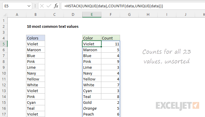
We are getting close to a solution, but we still need to reorder the list to show the highest counts first, and drop all but the top 10 counts.
Sort by count
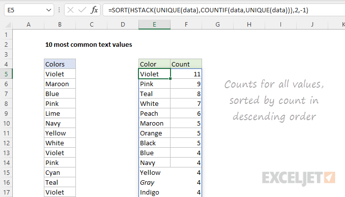
To sort the table by count, we can use the SORT function like this:
=SORT(HSTACK(UNIQUE(data),COUNTIF(data,UNIQUE(data))),2,-1)
Now we have the values sorted by count in descending order:
Top 10 values by count
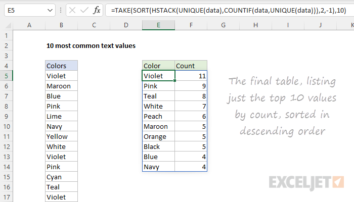
The final step is to remove all but the top 10 values. The easiest way to do this is with the TAKE function , which is designed to extract rows and columns from arrays. In this case, we want the first 10 rows, so we provide 10 for rows:
=TAKE(SORT(HSTACK(UNIQUE(data),COUNTIF(data,UNIQUE(data))),2,-1),10)
The screen below shows the output of this formula:
Optimize
The formula above works fine, but it is a bit inefficient, since UNIQUE values are calculated twice. This might impact performance in larger sets of data. To streamline the formula, we can use the LET function . The LET function is used to declare and assign values to variables. In this case, we can use LET like this:
=LET(u,UNIQUE(data),TAKE(SORT(HSTACK(u,COUNTIF(data,u)),2,-1),10))
Here, we use UNIQUE to get unique values and assign the result to a variable named u . Then we replace UNIQUE(data) with u where it occurs in the formula. The result is that UNIQUE values are calculated just one time.
Explanation
In this example, the goal is to create initials or acronyms with a formula using the data in column B as the source text. The formula should parse the text in column B, build a list of capital letters used to start words and join the capital letters together in a single text string. The article below explains 3 ways to do this. The first two methods require a current version of Excel. The last (and more complex method) is an array formula that will work in Excel 2019.
Modern formula #1
In the worksheet shown, the formula in cell D5 looks like this:
=LET(
text,B5,
chars,LEFT(TEXTSPLIT(text," ")),
codes,CODE(chars),
capitals,FILTER(chars,(codes>=65)*(codes<=90)),
TEXTJOIN("",1,capitals)
)
In brief, this formula splits the text in cell B5 into words, extracts the first letter of each word, removes all but the capital letters, and concatenates the result into a single string. The details work like this:
First, we use the LET Function to define four named variables ( text , chars , codes , capitals ) to make the formula easier to read and modify, as well as more efficient. The text variable is assigned the value in cell B5, and serves as the source text from which the capital letters will be extracted. Next, we assign a value to chars with this code:
LEFT(TEXTSPLIT(text," "))
The TEXTSPLIT function splits the text into an array of words using spaces (" “) as the delimiter . Next, the LEFT function extracts the first character from each word in the array created by TEXTSPLIT. The final result is an array of the first letters of each word.
Next, we create a value for codes using the CODE function :
CODE(chars)
Here, CODE returns a numeric ASCII value for each character in the chars array. The result is an array of ASCII numbers. We now have what we need to isolate capital letters only. This is done with the FILTER function :
FILTER(chars,(codes>=65)*(codes<=90))
The FILTER function filters the chars array to include only those characters whose codes are between 65 and 90, which correspond to the uppercase letters (A-Z) in ASCII. The result from FILTER is an array that contains only the capital letters that appear at the beginning of a word. This array is the value assigned to the variable capitals.
Finally, the formula concatenates the capital letters in capitals into a single text string using the TEXTJOIN function . The delimiter is set to an empty string (”"), so no additional characters are inserted. The ignore_empty argument is given as 1 so that TEXTJOIN will ignore any empty values in the capitals array.
Modern formula #2
The formula below shows another way to solve this problem in a modern version of Excel:
=LET(
text,B5,
chars,MID(text,SEQUENCE(LEN(text)),1),
codes,CODE(chars),
capitals,FILTER(chars,(codes>= 65)*(codes<= 90)),
TEXTJOIN("",1,capitals)
)
As above, the LET function is used to declare variables, which are the same four as above: text , chars , codes , and capitals . The value for text comes from cell B5, and serves as the source text for the formula. The value for chars is defined by the following snippet:
MID(text,SEQUENCE(LEN(text)),1)
This is a fairly common method in more advanced Excel formulas to convert a text string to an array of characters . The result is an array of every character in the source text. Next, we use the FILTER function to preserve only capital letters as before:
FILTER(chars,(codes>= 65)*(codes<= 90))
The resulting array contains all the capital letters in text. Finally, we use the TEXTJOIN function to join the letters together:
TEXTJOIN("",1,capitals)
The main thing to note in this approach is that we don’t bother with words, we simply collect and filter all the characters in the source text . That means a capital letter in any location will survive and appear in the final result.
Legacy Excel solution
The formulas above work well and I recommend you use them in a current version of Excel. I leave the example below mainly as a historical reminder of the state of Excel formulas not so long ago. Solving problems like this used to require insanely complex formulas because many key functions (i.e. TEXTSPLIT, FILTER, SEQUENCE, UNIQUE, SORT, etc.) were not available. As a result, the workarounds were ridiculously complicated.
Older versions of Excel do not contain TEXTSPLIT or FILTER. However, if you have Excel 2019, you have the TEXTJOIN function which can be used to solve this problem with a much more complex formula like this:
=TEXTJOIN("",1,IF(ISNUMBER(MATCH(CODE(MID(B5,ROW(INDIRECT("1:"&LEN(B5))),1)),ROW(INDIRECT("65:90")),0)),MID(B5,ROW(INDIRECT("1:"&LEN(B5))),1),""))
Note: this is a traditional array formula and must be entered with control + shift + enter.
Working from the inside out, the MID function is used to cast the string into an array of individual letters:
MID(B5,ROW(INDIRECT("1:"&LEN(B5))),1)
In this part of the formula, MID , ROW , INDIRECT , and LEN are used to convert a string to an array of letters, as described here . MID returns an array of all characters in the text.
{"W";"i";"l";"l";"i";"a";"m";" ";"S";"h";"a";"k";"e";"s";"p";"e";"a";"r";"e"}
This array is fed into the CODE function , which outputs an array of numeric ASCII codes, one for each letter. Separately, ROW and INDIRECT are used to create another numeric array:
ROW(INDIRECT("65:90")
This is the clever bit. The numbers 65 to 90 correspond to the ASCII codes for all capital letters between A-Z. This array goes into the MATCH function as the lookup array, and the original array of ASCII codes is provided as the lookup value.
MATCH then returns either a number (based on a position) or the #N/A error. Numbers represent capital letters, so the ISNUMBER function is used together with the IF function to filter results. Only characters whose ASCII code is between 65 and 90 will make it into the final array, which is then reassembled with the TEXTJOIN function to create the final abbreviation or acronym.
