Below is a brief overview of about 100 important Excel functions you should know, with links to detailed examples. We also have a large list of example formulas , a more complete list of Excel functions , and video training . If you are new to Excel formulas, see this introduction .
Note: Excel now includes Dynamic Array formulas , and almost 50 new functions .
Download: 101 Excel Functions PDF
Date and Time Functions
Excel provides many functions to work with dates and times .
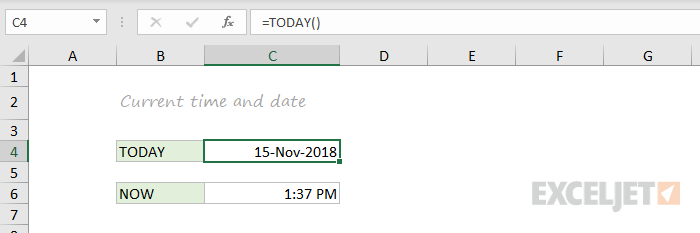
NOW and TODAY
You can get the current date with the TODAY function and the current date and time with the NOW Function . Technically, the NOW function returns the current date and time, but you can format as time only, as seen below:
TODAY() // returns current date
NOW() // returns current time
Note: these are volatile functions and will recalculate with every worksheet change. If you want a static value, use date and time shortcuts.
DAY, MONTH, YEAR, and DATE
You can use the DAY, MONTH , and YEAR functions to disassemble any date into its raw components, and the DATE function to put things back together again.

=DAY("14-Nov-2018") // returns 14
=MONTH("14-Nov-2018") // returns 11
=YEAR("14-Nov-2018") // returns 2018
=DATE(2018,11,14) // returns 14-Nov-2018
HOUR, MINUTE, SECOND, and TIME
Excel provides a set of parallel functions for times. You can use the HOUR , MINUTE , and SECOND functions to extract pieces of a time, and you can assemble a TIME from individual components with the TIME function .

=HOUR("10:30") // returns 10
=MINUTE("10:30") // returns 30
=SECOND("10:30") // returns 0
=TIME(10,30,0) // returns 10:30
DATEDIF and YEARFRAC
You can use the DATEDIF function to get time between dates in years, months, or days. DATEDIF can also be configured to get total time in “normalized” denominations, i.e. “2 years and 6 months and 27 days”.

Use YEARFRAC to get fractional years:

=YEARFRAC("14-Nov-2018","10-Jun-2021") // returns 2.57
EDATE and EOMONTH
A common task with dates is to shift a date forward (or backward) by a given number of months. You can use the EDATE and EOMONTH functions for this. EDATE moves by month and retains the day. EOMONTH works the same way, but always returns the last day of the month.

EDATE(date,6) // 6 months forward
EOMONTH(date,6) // 6 months forward (end of month)
WORKDAY and NETWORKDAYS
To figure out a date n working days in the future, you can use the WORKDAY function . To calculate the number of workdays between two dates, you can use NETWORKDAYS .

WORKDAY(start,n,holidays) // date n workdays in future
Video: How to calculate due dates with WORKDAY

NETWORKDAYS(start,end,holidays) // number of workdays between dates
Note: Both functions automatically skip weekends (Saturday and Sunday) and will also skip holidays, if provided. If you need more flexibility on what days are considered weekends, see the WORKDAY.INTL function and NETWORKDAYS.INTL function .
WEEKDAY and WEEKNUM
To figure out the day of week from a date, Excel provides the WEEKDAY function . WEEKDAY returns a number between 1-7 that indicates Sunday, Monday, Tuesday, etc. Use the WEEKNUM function to get the week number in a given year.
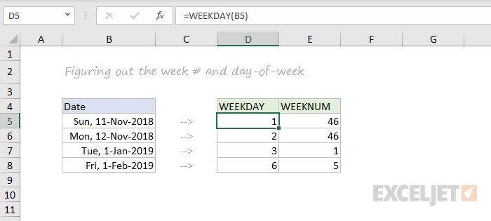
=WEEKDAY(date) // returns a number 1-7
=WEEKNUM(date) // returns week number in year
Engineering
CONVERT
Most Engineering functions are pretty technical…you’ll find a lot of functions for complex numbers in this section. However, the CONVERT function is quite useful for everyday unit conversions. You can use CONVERT to change units for distance, weight, temperature, and much more.

=CONVERT(72,"F","C") // returns 22.2
Information Functions
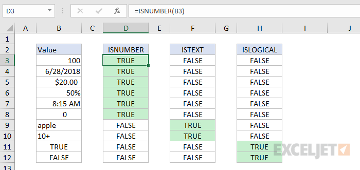
ISBLANK, ISERROR, ISNUMBER, and ISFORMULA
Excel provides many functions for checking the value in a cell, including ISNUMBER , ISTEXT , ISLOGICAL , ISBLANK , ISERROR , and ISFORMULA These functions are sometimes called the “IS” functions, and they all return TRUE or FALSE based on a cell’s contents.

Excel also has ISODD and ISEVEN functions that will test a number to see if it’s even or odd.
By the way, the green fill in the screenshot above is applied automatically with a conditional formatting formula.
Logical Functions
Excel’s logical functions are a key building block of many advanced formulas. Logical functions return the boolean values TRUE or FALSE. If you need a primer on logical formulas, t his video goes through many examples .
AND, OR and NOT
The core of Excel’s logical functions are the AND function , the OR function , and the NOT function . In the screen below, each of these function is used to run a simple test on the values in column B:
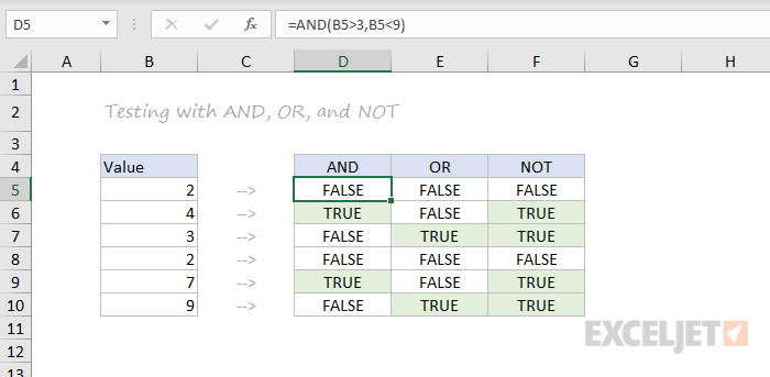
=AND(B5>3,B5<9)
=OR(B5=3,B5=9)
=NOT(B5=2)
- Video: How to build logical formulas
- Guide: 50 examples of formula criteria
IFERROR and IFNA
The IFERROR function and IFNA function can be used as a simple way to trap and handle errors. In the screen below, VLOOKUP is used to retrieve cost from a menu item. Column F contains just a VLOOKUP function , with no error handling. Column G shows how to use IFNA with VLOOKUP to display a custom message when an unrecognized item is entered.

=VLOOKUP(E5,menu,2,0) // no error trapping
=IFNA(VLOOKUP(E5,menu,2,0),"Not found") // catch errors
Whereas IFNA only catches an #N/A error, the IFERROR function will catch any formula error.
IF and IFS functions
The IF function is one of the most used functions in Excel. In the screen below, IF checks test scores and assigns “pass” or “fail”:

Multiple IF functions can be nested together to perform more complex logical tests.
New in Excel 2019 and Excel 365 , the IFS function can run multiple logical tests without nesting IFs .

=IFS(C5<60,"F",C5<70,"D",C5<80,"C",C5<90,"B",C5>=90,"A")
Lookup and Reference Functions
VLOOKUP and HLOOKUP
Excel offers a number of functions to lookup and retrieve data. Most famous of all is VLOOKUP :

=VLOOKUP(C5,$F$5:$G$7,2,TRUE)
More: 23 things to know about VLOOKUP .
HLOOKUP works like VLOOKUP , but expects data arranged horizontally:

=HLOOKUP(C5,$G$4:$I$5,2,TRUE)
INDEX and MATCH
For more complicated lookups, INDEX and MATCH offers more flexibility and power:

=INDEX(C5:E12,MATCH(H4,B5:B12,0),MATCH(H5,C4:E4,0))
Both the I NDEX function and the MATCH function are powerhouse functions that turn up in all kinds of formulas.
More: How to use INDEX and MATCH
LOOKUP
The LOOKUP function has default behaviors that make it useful when solving certain problems. LOOKUP assumes values are sorted in ascending order and always performs an approximate match. When LOOKUP can’t find a match, it will match the next smallest value. In the example below we are using LOOKUP to find the last entry in a column:

ROW and COLUMN
You can use the ROW function and COLUMN function to find row and column numbers on a worksheet. Notice both ROW and COLUMN return values for the current cell if no reference is supplied:

The row function also shows up often in advanced formulas that process data with relative row numbers .
ROWS and COLUMNS
The ROWS function and COLUMNS function provide a count of rows in a reference. In the screen below, we are counting rows and columns in an Excel Table named “Table1”.
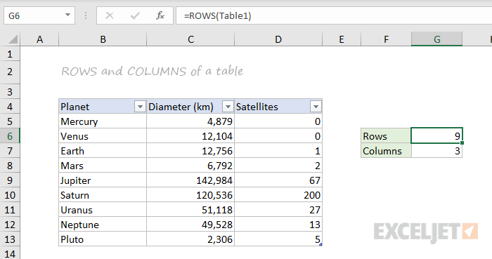
Note ROWS returns a count of data rows in a table, excluding the header row. By the way, here are 23 things to know about Excel Tables .
HYPERLINK
You can use the HYPERLINK function to construct a link with a formula. Note HYPERLINK lets you build both external links and internal links:
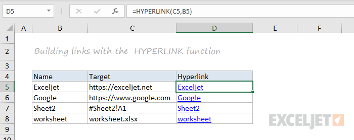
=HYPERLINK(C5,B5)
GETPIVOTDATA
The GETPIVOTDATA function is useful for retrieving information from existing pivot tables.
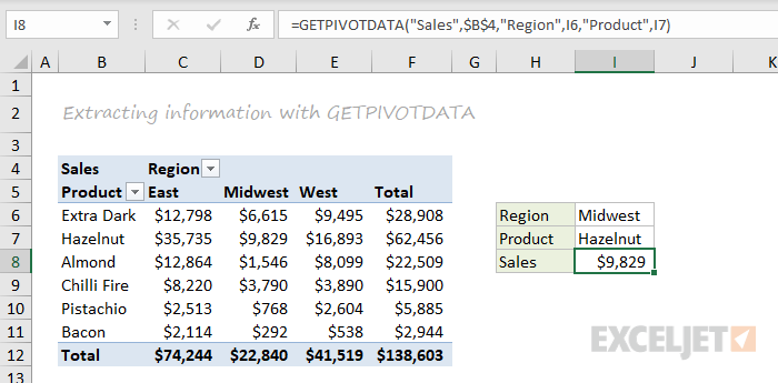
=GETPIVOTDATA("Sales",$B$4,"Region",I6,"Product",I7)
CHOOSE
The CHOOSE function is handy any time you need to make a choice based on a number:

=CHOOSE(2,"red","blue","green") // returns "blue"
Video: How to use the CHOOSE function
TRANSPOSE
The TRANSPOSE function gives you an easy way to transpose vertical data to horizontal, and vice versa.
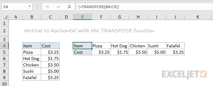
{=TRANSPOSE(B4:C9)}
Note: TRANSPOSE is a formula and is, therefore, dynamic. If you just need to do a one-time transpose operation, use Paste Special instead.
OFFSET
The OFFSET function is useful for all kinds of dynamic ranges. From a starting location, it lets you specify row and column offsets, and also the final row and column size. The result is a range that can respond dynamically to changing conditions and inputs. You can feed this range to other functions, as in the screen below, where OFFSET builds a range that is fed to the SUM function :
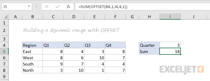
=SUM(OFFSET(B4,1,I4,4,1)) // sum of Q3
INDIRECT
The INDIRECT function allows you to build references as text. This concept is a bit tricky to understand at first, but it can be useful in many situations. Below, we are using INDIRECT to get values from cell A1 in 5 different worksheets. Each reference is dynamic. If a sheet name changes, the reference will update.

=INDIRECT(B5&"!A1") // =Sheet1!A1
The INDIRECT function is also used to “lock” references so they won’t change, when rows or columns are added or deleted. For more details, see linked examples at the bottom of the INDIRECT function page .
Caution: both OFFSET and INDIRECT are volatile functions and can slow down large or complicated spreadsheets.
STATISTICAL Functions
COUNT and COUNTA
You can count numbers with the COUNT function and non-empty cells with COUNTA . You can count blank cells with COUNTBLANK , but in the screen below we are counting blank cells with COUNTIF , which is more generally useful.

=COUNT(B5:F5) // count numbers
=COUNTA(B5:F5) // count numbers and text
=COUNTIF(B5:F5,"") // count blanks
COUNTIF and COUNTIFS
For conditional counts, the COUNTIF function can apply one criteria. The COUNTIFS function can apply multiple criteria at the same time:

=COUNTIF(C5:C12,"red") // count red
=COUNTIF(F5:F12,">50") // count total > 50
=COUNTIFS(C5:C12,"red",D5:D12,"TX") // red and tx
=COUNTIFS(C5:C12,"blue",F5:F12,">50") // blue > 50
Video: How to use the COUNTIF function
SUM, SUMIF, SUMIFS
To sum everything, use the SUM function . To sum conditionally, use SUMIF or SUMIFS. Following the same pattern as the counting functions, the SUMIF function can apply only one criteria while the SUMIFS function can apply multiple criteria.

=SUM(F5:F12) // everything
=SUMIF(C5:C12,"red",F5:F12) // red only
=SUMIF(F5:F12,">50") // over 50
=SUMIFS(F5:F12,C5:C12,"red",D5:D12,"tx") // red & tx
=SUMIFS(F5:F12,C5:C12,"blue",F5:F12,">50") // blue & >50
Video: How to use the SUMIF function
AVERAGE, AVERAGEIF, and AVERAGEIFS
Following the same pattern, you can calculate an average with AVERAGE , AVERAGEIF , and AVERAGEIFS .

=AVERAGE(F5:F12) // all
=AVERAGEIF(C5:C12,"red",F5:F12) // red only
=AVERAGEIFS(F5:F12,C5:C12,"red",D5:D12,"tx") // red and tx
MIN, MAX, LARGE, SMALL
You can find largest and smallest values with MAX and MIN , and nth largest and smallest values with LARGE and SMALL . In the screen below, data is the named range C5:C13, used in all formulas.

=MAX(data) // largest
=MIN(data) // smallest
=LARGE(data,1) // 1st largest
=LARGE(data,2) // 2nd largest
=LARGE(data,3) // 3rd largest
=SMALL(data,1) // 1st smallest
=SMALL(data,2) // 2nd smallest
=SMALL(data,3) // 3rd smallest
Video: How to find the nth smallest or largest value
MINIFS, MAXIFS
The MINIFS and MAXIFS . These functions let you find minimum and maximum values with conditions:

=MAXIFS(D5:D15,C5:C15,"female") // highest female
=MAXIFS(D5:D15,C5:C15,"male") // highest male
=MINIFS(D5:D15,C5:C15,"female") // lowest female
=MINIFS(D5:D15,C5:C15,"male") // lowest male
Note: MINIFS and MAXIFS are new in Excel via Office 365 and Excel 2019.
MODE
The MODE function returns the most commonly occurring number in a range:

=MODE(B5:G5) // returns 1
RANK
To rank values largest to smallest, or smallest to largest, use the RANK function :

Video: How to rank values with the RANK function
MATH Functions
ABS
To change negative values to positive use the ABS function .

=ABS(-134.50) // returns 134.50
RAND and RANDBETWEEN
Both the RAND function and RANDBETWEEN function can generate random numbers on the fly. RAND creates long decimal numbers between zero and 1. RANDBETWEEN generates random integers between two given numbers.

=RAND() // between zero and 1
=RANDBETWEEN(1,100) // between 1 and 100
ROUND, ROUNDUP, ROUNDDOWN, INT
To round values up or down, use the ROUND function . To force rounding up to a given number of digits, use ROUNDUP . To force rounding down, use ROUNDDOWN . To discard the decimal part of a number altogether, use the INT function .

=ROUND(11.777,1) // returns 11.8
=ROUNDUP(11.777) // returns 11.8
=ROUNDDOWN(11.777,1) // returns 11.7
=INT(11.777) // returns 11
MROUND, CEILING, FLOOR
To round values to the nearest multiple use the MROUND function . The FLOOR function and CEILING function also round to a given multiple. FLOOR forces rounding down, and CEILING forces rounding up.

=MROUND(13.85,.25) // returns 13.75
=CEILING(13.85,.25) // returns 14
=FLOOR(13.85,.25) // returns 13.75
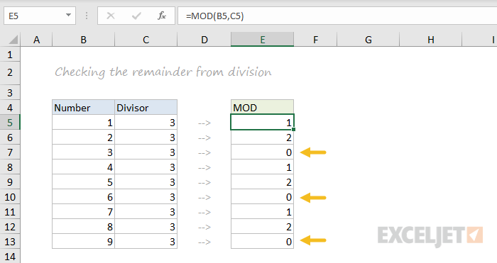
MOD
The MOD function returns the remainder after division. This sounds boring and geeky, but MOD turns up in all kinds of formulas, especially formulas that need to do something “every nth time”. In the screen below, you can see how MOD returns zero every third number when the divisor is 3:
SUMPRODUCT
The SUMPRODUCT function is a powerful and versatile tool when dealing with all kinds of data. You can use SUMPRODUCT to easily count and sum based on criteria, and you can use it in elegant ways that just don’t work with COUNTIFS and SUMIFS. In the screen below, we are using SUMPRODUCT to count and sum orders in March. See the SUMPRODUCT page for details and links to many examples.
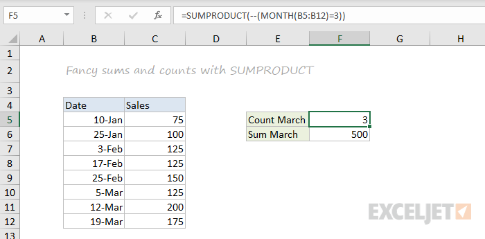
=SUMPRODUCT(--(MONTH(B5:B12)=3)) // count March
=SUMPRODUCT(--(MONTH(B5:B12)=3),C5:C12) // sum March
SUBTOTAL
The SUBTOTAL function is an “aggregate function” that can perform a number of operations on a set of data. All told, SUBTOTAL can perform 11 operations, including SUM, AVERAGE, COUNT, MAX, MIN, etc. (see this page for the full list). The key feature of SUBTOTAL is that it will ignore rows that have been “filtered out” of an Excel Table , and, optionally, rows that have been manually hidden. In the screen below, SUBTOTAL is used to count and sum only the 7 visible rows in the table:

=SUBTOTAL(3,B5:B14) // returns 7
=SUBTOTAL(9,F5:F14) // returns 9.54
AGGREGATE
Like SUBTOTAL, the AGGREGATE function can also run a number of aggregate operations on a set of data and can optionally ignore hidden rows. The key differences are that AGGREGATE can run more operations (19 total) and can also ignore errors.
In the screen below, AGGREGATE is used to perform MIN, MAX, LARGE and SMALL operations while ignoring errors. Normally, the error in cell B9 would prevent these functions from returning a result. See this page for a full list of operations AGGREGATE can perform.
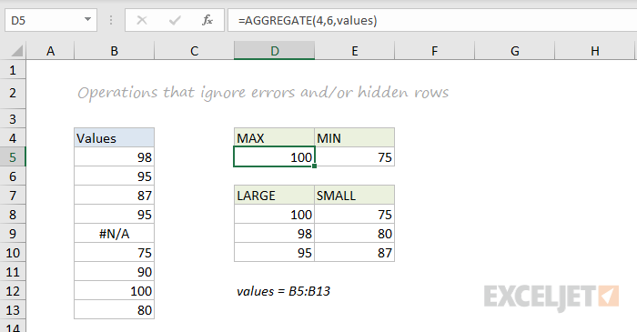
=AGGREGATE(4,6,values) // MAX ignore errors, returns 100
=AGGREGATE(5,6,values) // MIN ignore errors, returns 75
TEXT Functions
LEFT, RIGHT, MID
To extract characters from the left, right, or middle of text, use LEFT , RIGHT , and MID functions :

=LEFT("ABC-1234-RED",3) // returns "ABC"
=MID("ABC-1234-RED",5,4) // returns "1234"
=RIGHT("ABC-1234-RED",3) // returns "RED"
LEN
The LEN function will return the length of a text string. LEN shows up in a lot of formulas that count words or characters .

FIND, SEARCH
To look for specific text in a cell, use the FIND function or SEARCH function . These functions return the numeric position of matching text, but SEARCH allows wildcards and FIND is case-sensitive. Both functions will throw an error when text is not found, so wrap in the ISNUMBER function to return TRUE or FALSE ( example here ).

=FIND("Better the devil you know","devil") // returns 12
=SEARCH("This is not my beautiful wife","bea*") // returns 12
REPLACE, SUBSTITUTE
To replace text by position, use the REPLACE function . To replace text by matching, use the SUBSTITUTE function . In the first example, REPLACE removes the two asterisks (**) by replacing the first two characters with an empty string (""). In the second example, SUBSTITUTE removes all hash characters (#) by replacing “#” with “”.
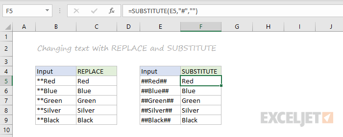
=REPLACE("**Red",1,2,"") // returns "Red"
=SUBSTITUTE("##Red##","#","") // returns "Red"
CODE, CHAR
To figure out the numeric code for a character, use the CODE function . To translate the numeric code back to a character, use the CHAR function . In the example below, CODE translates each character in column B to its corresponding code. In column F, CHAR translates the code back to a character.
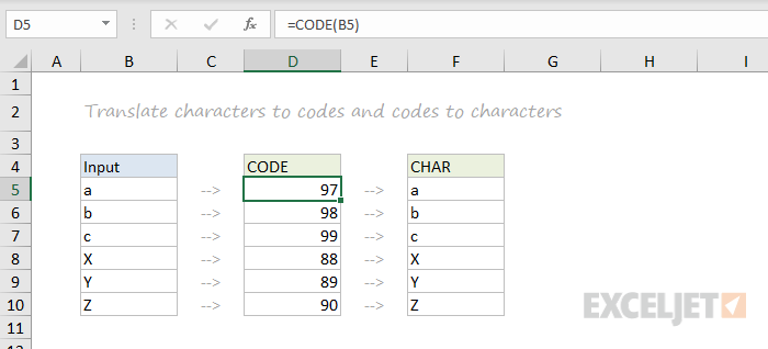
=CODE("a") // returns 97
=CHAR(97) // returns "a"
Video: How to use the CODE and CHAR functions
TRIM, CLEAN
To get rid of extra space in text, use the TRIM function . To remove line breaks and other non-printing characters, use CLEAN .

=TRIM(A1) // remove extra space
=CLEAN(A1) // remove line breaks
Video: How to clean text with TRIM and CLEAN
CONCAT, TEXTJOIN, CONCATENATE
New in Excel via Office 365 are CONCAT and TEXTJOIN. The CONCAT function lets you concatenate (join) multiple values, including a range of values without a delimiter. The TEXTJOIN function does the same thing, but allows you to specify a delimiter and can also ignore empty values.
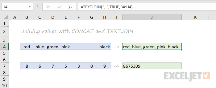
=TEXTJOIN(",",TRUE,B4:H4) // returns "red,blue,green,pink,black"
=CONCAT(B7:H7) // returns "8675309"
Excel also provides the CONCATENATE function , but it doesn’t offer special features. I wouldn’t bother with it and would instead concatenate directly with the ampersand (&) character in a formula.
EXACT
The EXACT function allows you to compare two text strings in a case-sensitive manner.

UPPER, LOWER, PROPER
To change the case of text, use the UPPER , LOWER , and PROPER function

=UPPER("Sue BROWN") // returns "SUE BROWN"
=LOWER("Sue BROWN") // returns "sue brown"
=PROPER("Sue BROWN") // returns "Sue Brown"
Video: How to change case with formulas
TEXT
Last but definitely not least is the TEXT function . The text function lets you apply number formatting to numbers (including dates, times, etc.) as text. This is especially useful when you need to embed a formatted number in a message, like “Sale ends on [date]”.
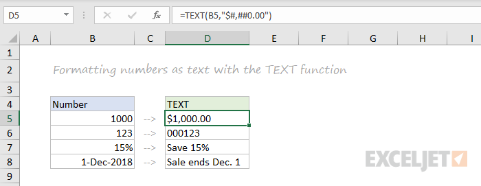
=TEXT(B5,"$#,##0.00")
=TEXT(B6,"000000")
="Save "&TEXT(B7,"0%")
="Sale ends "&TEXT(B8,"mmm d")
More: Detailed examples of custom number formatting .
Dynamic Array functions
Dynamic arrays are new in Excel 365 , and are a major upgrade to Excel’s formula engine. As part of the dynamic array update, Excel includes new functions which directly leverage dynamic arrays to solve problems that are traditionally hard to solve with conventional formulas. If you are using Excel 365, make sure you are aware of these new functions:
| Function | Purpose |
|---|---|
| FILTER | Filter data and return matching records |
| RANDARRAY | Generate array of random numbers |
| SEQUENCE | Generate array of sequential numbers |
| SORT | Sort range by column |
| SORTBY | Sort range by another range or array |
| UNIQUE | Extract unique values from a list or range |
| XLOOKUP | Modern replacement for VLOOKUP |
| XMATCH | Modern replacement for the MATCH function |
Video: New dynamic array functions in Excel (about 3 minutes).
Quick navigation
ABS , AGGREGATE , AND , AVERAGE , AVERAGEIF , AVERAGEIFS , CEILING , CHAR , CHOOSE , CLEAN , CODE , COLUMN , COLUMNS , CONCAT , CONCATENATE , CONVERT , COUNT , COUNTA , COUNTBLANK , COUNTIF , COUNTIFS , DATE , DATEDIF , DAY , EDATE , EOMONTH , EXACT , FIND , FLOOR , GETPIVOTDATA , HLOOKUP , HOUR , HYPERLINK , IF , IFERROR , IFNA , IFS , INDEX , INDIRECT , INT , ISBLANK , ISERROR , ISEVEN , ISFORMULA , ISLOGICAL , ISNUMBER , ISODD , ISTEXT , LARGE , LEFT , LEN , LOOKUP , LOWER , MATCH , MAX , MAXIFS , MID , MIN , MINIFS , MINUTE , MOD , MODE , MONTH , MROUND , NETWORKDAYS , NOT , NOW , OFFSET , OR , PROPER , RAND , RANDBETWEEN , RANK , REPLACE , RIGHT , ROUND , ROUNDDOWN , ROUNDUP , ROW , ROWS , SEARCH , SECOND , SMALL , SUBSTITUTE , SUBTOTAL , SUM , SUMIF , SUMIFS , SUMPRODUCT , TEXT , TEXTJOIN , TIME , TODAY , TRANSPOSE , TRIM , UPPER , VLOOKUP , WEEKDAY , WEEKNUM , WORKDAY , YEAR , YEARFRAC
One of the most important skills for building formulas is creating criteria – the part of a formula that decides what to include or exclude in a calculation. However, it can be surprisingly tricky to build effective criteria because it requires a good understanding of how Excel handles data. If you’ve ever spent an afternoon troubleshooting a formula that seems like it should “just work”, you know what I mean :)
This guide aims to help you build formulas that work the first time.
Note: language mavens will point out that “criterion” is singular and “criteria” is plural, but I’m going to use “criteria” in both cases to keep things simple.
Function names on dark backgrounds below are links to more information.
What do criteria do?
Among other things, criteria:
- Direct logical flow with IF/THEN logic
- Restrict processing to matching values only
- Create conditional sums and counts
- Filter data to exclude irrelevant information
- Trigger conditional formatting rules
To help set the stage, let’s look at three examples of criteria in action.
Example #1
In the screen below, F3 contains this formula:
=IF(E3>30,"Yes","No")

Translation: If the value in E3 is greater than 30, return “Yes”, otherwise return “No”.
Here, E3>30 is the criteria, used inside IF to determine if the formula should return “Yes” or “No” for each invoice.
Example #2
In the next example, D3 contains this formula:
=IF(OR(B3="red",B3="green"),C3*1.1,C3)
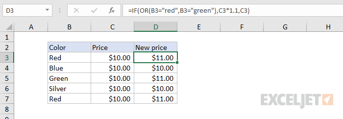
Translation: if B3 is either “red” or “green”, increase the price by 10%. Otherwise, return the original price.
Example #3
In this example, the SUMIFS function is used to sum the total only when the color is “red”:
=SUMIFS(E3:E7,B3:B7,"red")
<img loading=“lazy” src=“https://exceljet.net/sites/default/files/styles/original_with_watermark/public/images/articles/inline/formula%20criteria%20example%203.png?itok=qbFid8fV" onerror=“this.onerror=null;this.src=‘https://blogger.googleusercontent.com/img/a/AVvXsEhe7F7TRXHtjiKvHb5vS7DmnxvpHiDyoYyYvm1nHB3Qp2_w3BnM6A2eq4v7FYxCC9bfZt3a9vIMtAYEKUiaDQbHMg-ViyGmRIj39MLp0bGFfgfYw1Dc9q_H-T0wiTm3l0Uq42dETrN9eC8aGJ9_IORZsxST1AcLR7np1koOfcc7tnHa4S8Mwz_xD9d0=s16000';" alt=“Formula criteria example #2 - SUMIF when color is “red” - 56”>
Translation: sum values in E3:E7 when the value in B3:B7 is “red”.
Criteria Basics
This section covers the building blocks of formula criteria and some simple ways to verify that criteria are performing as expected.
What are criteria?
Criteria are logical expressions that return TRUE or FALSE, or their numerical equivalents, 1 or 0.
That’s it.
The trick is to construct criteria in a way so that they only return TRUE when the test meets your exact criteria. In all other cases, criteria should return FALSE or zero. If you can master this one idea, you have the foundation to build and understand many advanced formulas.
Logical operators
Criteria often make use of the logical operators listed in the table below.
| Operator | Meaning | Example |
|---|---|---|
| = | Equal to | =A1=10 |
| <> | Not equal to | =A1<>10 |
| > | Greater than | =A1>100 |
| < | Less than | =A1<100 |
| >= | Greater than or equal to | =A1>=75 |
| <= | Less than or equal to | =A1<=0 |
Logical operators can be combined in various ways, as seen in the examples below.
Logical functions
Excel has several so-called “logical functions” that can be used to construct and utilize conditions. The table below lists the key logical functions.
| Function | Purpose |
|---|---|
| IF | Test one condition; direct logical flow |
| IFS | Test multiple conditions; direct logical flow |
| NOT | Reverse criteria or results |
| AND | Test multiple conditions, return TRUE if all are TRUE |
| OR | Test multiple conditions, return TRUE if at least one is TRUE |
| XOR | Exclusive OR – return TRUE if one or the other, not both |
| IFERROR | Trap errors and return alternative results |
Multiple criteria
Naturally, there are many cases where you will want to use multiple criteria. In simple situations, you can use the AND, OR, and NOT functions. Here are a few examples:
=AND(A1>0,A1<10) // greater than 0 and less than 10
=OR(A1="red",A1="blue") // red or blue
=NOT(OR(A1="red",A1="blue")) // not red or blue
=AND(ISNUMBER(A1),A1>100) // number greater than 100
Wildcards
Excel provides three “wildcards” for matching text in formulas:
| Character | Name | Purpose |
|---|---|---|
| * | Asterisk | Match zero or more characters |
| ? | Question mark | Match any one character |
| ~ | Tilde | Match literal wildcard |
Wildcards can be used alone or combined to get a variety of matching behaviors:
| Usage | Behavior | Will match |
|---|---|---|
| ? | Any one character | “A”, “B”, “c”, “z”, etc. |
| ?? | Any two characters | “AA”, “AZ”, “zz”, etc. |
| ??? | Any three characters | “Jet”, “AAA”, “ccc”, etc. |
| * | Any characters | “apple”, “APPLE”, “A100”, etc. |
| *th | Ends in “th” | “bath”, “fourth”, etc. |
| c* | Starts with “c” | “Cat”, “CAB”, “cindy”, “candy”, etc. |
| ?* | At least one character | “a”, “b”, “ab”, “ABCD”, etc. |
| ???-?? | 5 characters with a hyphen | “ABC-99”,“100-ZT”, etc. |
| *~? | Ends with a question mark | “Hello?”, “Anybody home?”, etc. |
| xyz | Contains “xyz” | “code is XYZ”, “100-XYZ”, “XyZ90”, etc. |
Here are a few examples of using wildcards for criteria in the COUNTIFS function.
=COUNTIFS(A1:A100,"*red*") // count cells that contain "red"
=COUNTIFS(A1:A100, "www*") // count cells starting with "www"
=COUNTIFS(A1:A100,"?????") // count cells with 5 characters
Not all functions allow wildcards. Here is a list of common functions that do:
- AVERAGEIF , AVERAGEIFS
- COUNTIF , COUNTIFS
- SUMIF , SUMIFS
- VLOOKUP , HLOOKUP
- MATCH
- SEARCH
Notice the IF function is not on this list. To get wildcard behavior with IF, you can combine the SEARCH and ISNUMBER functions, as described below.
Testing criteria
The classic way to test criteria is to wrap them in the IF function. For example, to check for “red” or “blue”, we can wrap the OR function inside IF like this:
=IF(OR(B3="red",B3="blue"),"OK", "")
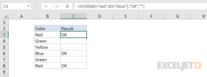
Translation: if the color is “red” or “blue”, return “OK”. Otherwise, return nothing.
However, you can also test criteria directly on the worksheet as a formula. Let’s say you want to process values that are 80 and higher. In the screen below, C3 contains this formula, copied down.
=B3>=80
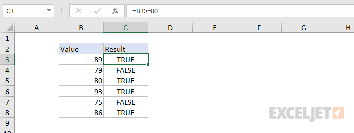
Translation: the value in B3 is greater than or equal to 80.
Without IF or another function, we only get a result of TRUE or FALSE, but it’s enough to verify criteria are working as expected.
Don’t be thrown off by the equals (=) sign when testing criteria as a formula. All Excel formulas must begin with an equals sign, so it must be included. Remove the equal sign when you move criteria into another formula.
Another way to test criteria is to use F9 to evaluate the criteria in place. Just carefully select a logical expression, and press F9. Excel will immediately evaluate the expression and display the result.
Video: How to use F9 to debug a formula .
Adding criteria to formulas
Of course, in most cases, you don’t want to return TRUE or FALSE to a cell, you want to return some other value based on criteria returning TRUE or FALSE. To do that, just remove the equal sign and add the criteria where needed in the formula.
In the example below, the formula C3 contains this formula, which uses the criteria above as the logical test inside IF:
=IF(B3>=80,"Pass","Fail")
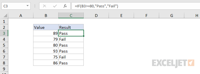
Translation: if the value in B3 is greater than or equal to 80, return “Pass”. Otherwise, return “Fail”.
See also: 23 tips for formulas ( video | article )
Criteria Examples
This section shows examples of how to build criteria to accomplish a variety of tasks for different kinds of content.
Blank or not blank
There are several ways you can check for blank or non-blank cells. To return TRUE if A1 is blank, you can use either:
=ISBLANK(A1)
=A1=""
To reverse the logic and check for non-blank cells, you can use:
=NOT(ISBLANK(A1))
=A1<>""
Another way to test for a blank cell is to count characters:
=LEN(A1)=0
If the count is zero, the cell is “blank”. This formula is useful when testing cells that may contain formulas that return empty strings (””). ISBLANK(A1) will return FALSE if a formula returns an empty string in A1, but LEN(A1)=0 will return TRUE.
Criteria for text
To return TRUE if a cell contains “red”, you can use:
=A1="red"
To reverse logic, you can use the NOT function or the “not equals to” operator (<>) like this:
=NOT(A1="red")
=A1<>"red"
Notice in each case the text IS enclosed in double quotes (e.g. “red”). If you don’t use quotes, Excel will think you are trying to reference a named range or a function and will return the #NAME error.
Criteria for numbers
To test if A1 is equal to 5, you can use criteria like this:
=A1=5 // TRUE if A1 equals 5
Here are some other examples of criteria to test numeric values:
=A1<100 // less than 100
=A1>=1 // greater than or equal to 1
=A1<>0 // not equal to zero
=AND(A1>0,A1<5) // greater than zero, less than 5
=MOD(A1,3)=0 // value is a multiple of 3
Notice numbers are NOT enclosed in double quotes. If you enclose a number in quotes, you are telling Excel to treat the number as text, which will make the criteria useless. Also, remember that number formatting in Excel affects display only, and does not change numeric data in any way. Do not include dollar signs ($), percent signs (%), or other formatting information when building criteria to test numbers.
Criteria for dates
Dates in Excel are just numbers, which means you are free to use ordinary math operations on dates if you like. With Order dates in column A and Delivery dates in column B, this formula in column C will mark delivery times greater than 3 days as “late”:
=IF((B2-A2)>3,"Late","")
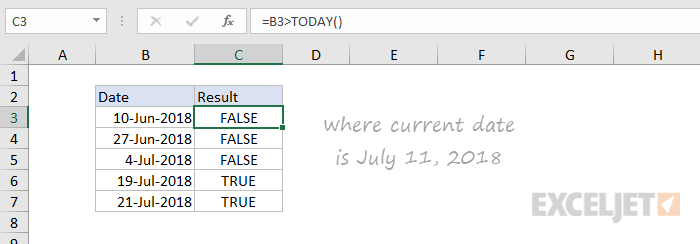
Excel also provides a large number of specific functions for working with dates. For example, to check if a date is “in the future” you can use the TODAY function like this:
=A1>TODAY()
To check if a date occurs in the next 30 days, the formula can be extended to:
=AND(A1>TODAY(),A1<=(TODAY()+30))
Translation: IF A2 is greater than today AND less than or equal today + 30 days, return TRUE.
Here are a few other examples of criteria for dates, assuming A1 contains a valid date:
=DAY(A1)>15 // greater than 15th
=MONTH(A1)=6 // month is June
=YEAR(A1) = 2019 // year is 2019
=WEEKDAY(A1)=2 // date is a Monday
The safest way to insert a valid date into criteria is to use the DATE function, which accepts year , month , and day as separate arguments. Here are a couple of examples:
=A1>DATE(2019,1,1) // after Jan. 1, 2019
=AND(A1>=DATE(2018,6,1),B4<=DATE(2018,8,31)) // Jun-Aug 2018
Criteria for times
Times are fractional numbers in Excel, so you can use simple math for time in some cases. For example, to check if a time in A1 is after 12:00 PM (more than 12 hours), you can use:
=A1>.5
This works because 1 day = 24 hours, so a half day = 12 hours.
For more granular work, Excel has special functions to extract time by component. For example, with the time 8:45 AM in cell A1:
=HOUR(A1) // returns 8
=MINUTE(A1) // returns 45
=SECOND(A1) // returns 0
The safest way to insert a time in criteria is to use the TIME function. Here are some examples:
=A1>TIME(9,15,0) // after 9:15 AM
=AND(A1>=TIME(9,0,0),A1<=TIME(17,0,0)) // 9 AM to 5 PM
Criteria for SUMIFS, COUNTIFS, etc.
The criteria for SUMIFS, COUNTIFS, AVERAGEIFS, and similar range-based functions follow slightly different rules. This is because the criteria are split into two parts (criteria range and criteria), and this impacts the syntax when criteria include operators.
Simple criteria based on equality don’t need special handling. The equals (=) operator is implied, so there’s no need to include it:
=COUNTIFS(A1:A100,10) // count cells equal to 10
=COUNTIFS(A1:A100,"red") // count cells that equal "red"
However, things change when we add operators:
=COUNTIFS(A1:A100,">10") // count cells greater than 10
=COUNTIFS(A1:A100,"<0") // count cells less than zero
Notice the quotes ("") around the criteria? These are required when criteria include an operator in these functions.
Criteria for data types
Excel allows three main data types: text, numbers, and logicals. Dates, times, percentages, and fractions are all just numbers with number formatting applied to change the way they are displayed. By default, numbers are right-aligned, text is left-aligned, and logical values are centered. However a user can override alignment manually, so this is not a good test of type.
Excel provides three functions you can use to check data types: ISTEXT, ISNUMBER, and ISLOGICAL. These functions return TRUE or FALSE. In the screen below, the cells D3, F3, and H3 contain these formulas, copied down:
=ISTEXT(B3)
=ISNUMBER(B3)
=ISLOGICAL(B3)
To use these functions as criteria, just place them in the correct location of a formula. For example, to check if A1 contains a number, you can use ISNUMBER as the logical test inside IF like this:
=IF(ISNUMBER(B3),"OK","Invalid")
Note: Formulas are not a data type, but you can check for formulas with the ISFORMULA function :
=ISFORMULA(A1) // TRUE if A1 contains formula
Getting fancy
The examples above show the fundamentals of using criteria in formulas, there are many ways to make criteria more sophisticated. This section explores a few techniques.
Making criteria variable
It is often useful to make criteria variable, by referencing a cell on the worksheet. For example, in the worksheet below, the passing score is in cell E3, and the formula to determine pass or fail looks like this:
=IF(B3>=$E$3,"Pass","Fail")
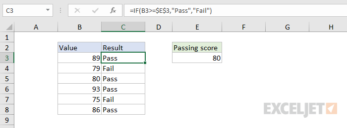
Placing the passing score in cell E3 makes it easy to change at any time without editing formulas. Note that the reference to $E$3 is absolute to prevent changes as the formula is copied down.
Making criteria variable in COUNTIFS, SUMIFS, etc.
As before, if criteria are testing for equality, no special handling is needed:
=COUNTIF(range,A1) // count cells equal to A1
However, if criteria include operators, you will need to use concatenation . For example, to count cells greater than A1, join “>” to “A1” like this:
=COUNTIF(range,">"&A1)
The concatenation runs first. If A1 contains the number 10, this is the formula after concatenation:
=COUNTIF(range,">10")
Notice the pattern is the same as explained earlier – if criteria includes operators, it must appear in quotes ("").
Here are more examples of using concatenation in criteria:
=COUNTIF(range,"<"&B1) // count less than value in B1
=COUNTIF(range,"<>"&"") // count not blank cells
=COUNTIF(range,"*"&B1&"*") // count contains text in B1
=COUNTIF(range,">"&TODAY()) // count dates in future
=COUNTIF(range,"<"&TODAY()+7) // count up to 7 days from today
Contains specific text
One tricky situation is when you want to test if a cell contains specific text. For functions that support wildcards (like COUNTIFS, SUMIFS, etc.), you can use wildcards to do this. For example, to count cells that contain “red” anywhere in a cell with COUNTIFS, you can use an asterisk like this:
=COUNTIFS(A1:A100,"*red*")
However, many other functions (like the IF function) don’t support wildcards. In that case, you can combine ISNUMBER and SEARCH to create logic that checks a cell for a partial match. In the screen below, D3 contains this formula:
=ISNUMBER(SEARCH(C3,B3))
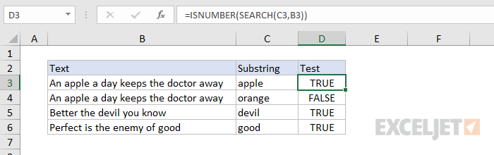
You can use this expression as criteria inside IF like this
=IF(ISNUMBER(SEARCH("red",A1)),"red", "")
Translation: if “red” is found anywhere in A1, return “red”.
This works because SEARCH returns a numeric position if “red” is found, and ISNUMBER returns TRUE. If not, SEARCH returns an error, and ISNUMBER returns FALSE. For more details, see this page .
Nested IFs
Nested IF formulas are often used to check multiple criteria and return multiple results. In general, the challenge is to build nested IFs so that the criteria appear in the right sequence. For example, here is a nested IF formula that assigns a letter grade based on a numeric score:
=IF(C5<64,"F",IF(C5<73,"D",IF(C5<85,"C",IF(C5<95,"B","A"))))
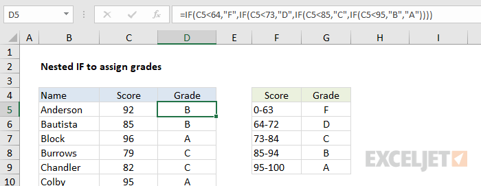
Notice we are testing for low scores first, then progressively higher scores.
More: 19 tips for nested IFs (with alternatives)
Array constants in criteria
Array constants are hard-coded arrays with fixed values like this: {“A”,“B”,“C”}. They can sometimes be used as criteria to create simple OR logic criteria. For example, in the screen below, cell F4 contains this formula:
=SUM(SUMIFS(C3:C7,B3:B7,{"red","gold"}))
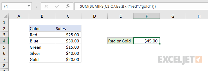
Translation: SUM sales where the color is “red” OR “gold”.
Because we give SUMIFS two values for criteria, it returns two results. The SUM function then returns the sum of the two results.
Simple array formula criteria
Array formulas are a complicated topic, but the criteria for simple array formulas can be quite simple. A classic example is using the IF function to “filter out” values that should be excluded, and then processing the result with another function.
In the screen below, the formula in G4 is:
{=MAX(IF(regions=F4,totals))}
where regions is the named range B3:B8 and totals is the named range D3:D8.
Note: this is an array formula and must be entered with control + shift + enter.
The result is the top value for each region.
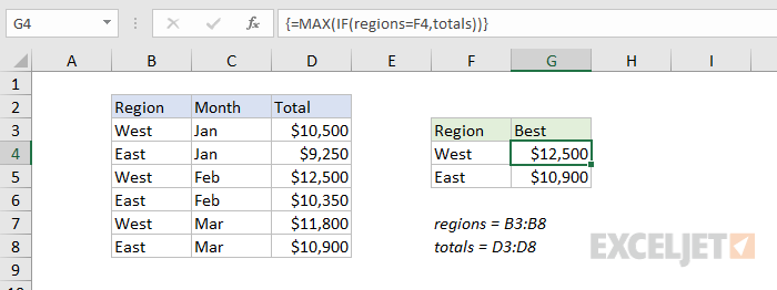
For criteria, we use the expression:
regions=F4
This compares all region values with “West” from F4, and returns the following array result in the logical test for IF:
{TRUE;FALSE;TRUE;FALSE;TRUE;FALSE}
The final array returned by IF looks like this:
{10500;FALSE;12500;FALSE;11800;FALSE}
Only values associated with the “West” region make it into the array. Values associated with the “East” region are FALSE.
The MAX function then returns the largest value in the array, ignoring all FALSE values.
Advanced formula criteria
Below are links to more advanced formula criteria examples. Each link has a screenshot and a full explanation.
- Count cells that contain errors
- Sum if value is equal to one of many
- COUNTIFS with multiple criteria and OR logic
- Get nth largest value with criteria
- Sum top n values with criteria
- INDEX and MATCH with multiple criteria
More formula resources
The following links contain more detailed information on Excel formulas:
- How to build logical formulas (video)
- 19 tips for nested IF formulas
- 30+ conditional formatting formulas
- Core Formula (paid training)
