A few days ago, I posted this conditional formatting puzzle :
Given a date, what formula will highlight other dates in the same month and year?

Here’s the list:
Option #1 - Extract with MONTH and YEAR and test with AND Option #2 - force dates to first of month and compare Option #3 - force dates to last of month and compare Option #4 - concatenate year and month and compare Option #5 - concatenate year and month with TEXT and compare
Download the practice worksheet attached below and try them out yourself. In the worksheet, cell E2 is named “date”.
If you need a quick recap on how to use a formula with conditional formatting, see: How to apply conditional formatting with a formula . Here is another article on Conditional formatting based on a different cell.
The purpose of these formulas is to automatically highlight dates in the table whenever the date in E2 changes.
Option #1- Extract with MONTH and YEAR and test with AND
The “obvious” solution (if you’re an Excel nerd :)) is one that uses the AND function along with MONTH and YEAR. It looks like this:
=AND(YEAR(B4)=YEAR(date),MONTH(B4)=MONTH(date))
This formula uses the AND function to test two conditions:
YEAR(B4)=YEAR(date) // is the year the same?
MONTH(B4)=MONTH(date) // is the month the same?
Both of these conditions use the equal sign to force a TRUE or FALSE result. If both return TRUE, AND returns TRUE and the conditional formatting is triggered.
Pros - intuitive, straightforward Cons - requires five function calls and four references
I also like this formula because it builds on simple functions that you absolutely need to know: MONTH, YEAR & AND.
Option #2- force dates to first of month and compare
Another interesting solution is to pull out the month and year from each date and use these values to build “first of the month” dates, which are then compared. The formula looks like this:
=DATE(YEAR(B4),MONTH(B4),1)=DATE(YEAR(date),MONTH(date),1)
There are two main parts of the formula. On the left of the equal sign, the formula extracts the year and month values from B4, then uses those values to create a new date with the day value hard-coded as 1. On the right, the same thing happens with the date in date ($E$2).
=DATE(YEAR(B4),MONTH(B4),1)=DATE(YEAR(date),MONTH(date),1)
=DATE(2015,2,1)=DATE(2015,6,1)
=42036=42156*
=FALSE
- 42036 is the date serial number for 1-Feb-2015 and 42156 is the serial number for 1-Jun-2015, which is how Excel evaluates the dates internally.
In each case, the year and month values are extracted, and used to create a new date where the day value is hard-coded as 1. Effectively, this ignores day completely by making it the same for each date.
Finally, the two dates are tested for equality.
Pros - fairly intuitive Cons - requires six function calls and four references
What I like about this formula is the creative thinking — the “trick” of forcing the day to 1. You’ll find these kind of tricks are everywhere in more complex Excel formulas.
Option #3 - force dates to last of month and compare
Similar to option #3, another clever idea from reader Eric Kalin is to force dates to “last of month” and compare. This is a nice solution because Excel has a dedicated function for getting the last day a month: EOMONTH. The formula looks like this:
=EOMONTH(B4,0)=EOMONTH(date,0)
This formula can be summarized like this: get the last of month using the date in B4 and compare it to the last day of month based on the date in $E$2.
Pros - compact and economical; just two function calls and two references Cons - need to know and understand EOMONTH
Overall, a very nice formula that stands out for its simplicity.
Option #4 - concatenate year and month and compare
Yet another approach is to extract and concatenate the year and month values for each date, then compare the result:
=MONTH(B4)&YEAR(B4)=MONTH(date)&YEAR(date)
This may not be a solution you’d think of initially, because the idea of concatenating numbers is a little weird.
If you concatenate, say, 11 (November) with the year 2015, you’ll get “112015”, which is likely not a value you’d recognize at first glance. However, to Excel, it’s just a string (text value), and Excel will be happy to compare it with any other string for you. So, here’s what the formula looks like for cell B4 and cell $E$2 as it’s solved:
=MONTH(B4)&YEAR(B4)=MONTH(date)&YEAR(date)
="22015"="62015"
=FALSE
Pros - logical and relatively compact (4 function calls) Cons - need to know about concatenation
Option #5 - concatenate year and month with TEXT and compare
Finally, here is another formula that relies on the idea of concatenating the month and year together. However, this formula uses the TEXT function and a custom number format, rather than concatenating manually with the ampersand (&) operator:
=TEXT(B4,"myyyy")=TEXT(date,"myyyy")
TEXT is a useful function that allows you to convert a number to text in the text format of your choice. In this case the format is the custom date format “myyyy”, which translates to: month number without leading zeros & 4-digit year.
Like #4 above, the result is the same as concatenating the month and year manually. Solving with B4 and date ($E$2):
=TEXT(B4,"myyyy")=TEXT(date,"myyyy")
="22015"="62015"
=FALSE
Pros - simple and compact (2 function calls) Cons - need to understand TEXT
What’s the best option?
Well, in many cases, the best option is the one you know :)
If you spend a lot of time with Excel formulas, you’ll notice an obsession (in yourself, and in others) with compact and elegant formulas. It’s hard not to be delighted by a clever and efficient formula. And it’s true that shorter formulas offer less chance of making a mistake, since you aren’t wrangling as many parentheses and references.
But all that said, Excel is a vehicle, not a destination. Unless you build models professionally, or analyze huge data sets (where efficiency really counts), your boss probably doesn’t care what formula you use as long as it gets the job done accurately, and is straightforward to understand.
Are you looking for more conditional formatting formulas ?
You’ve heard of data visualization, right? It’s the art and science of presenting data in a way so that people can “see” important information at a glance . Data visualization makes complex data more accessible and useful. In a world overflowing with data, it’s more valuable than ever.
Excel has a great tool for visualizing data called Conditional Formatting. If you work with data in Excel (and who doesn’t these days?) you’ll find it incredibly useful. By creating simple rules that highlight just the data you are interested in , you can spot key information very quickly.
To help get you started, and to give you some inspiration, here are some cool ways that you can use Excel conditional formatting to help you understand data faster.
Highlight duplicate or unique values
One of the handy ways you can use conditional formatting is to highlight duplicate or unique values quickly. Excel contains built-in rules to make both of these tasks easy.
For example, suppose you have this table of zip codes, and you want to highlight duplicate zip codes? With over 160 zip codes in the list, it’s almost impossible for the human eye to spot duplicate codes.

But using Conditional Formatting, you can just select the table and tell Excel to highlight duplicates using a built-in conditional formatting rule for duplicates:
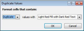
With just a few clicks, here is the result:

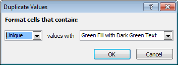
Alternately, suppose you have this table of names and you need to find only unique values (values that appear once)?

Good luck finding names that appear only once with just your eyes! However, using a built-in conditional formatting rule, you can find all unique names in less than 10 seconds:

Flipping the problem yet again, what if you wanted to find all names that appear at least 5 times? By creating a rule based on a formula:
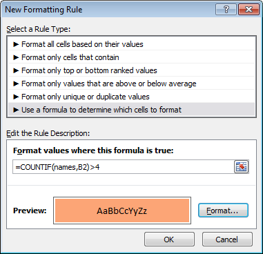
You can easily highlight names that appear at least 5 times:

The formula I’m using, with a named range “names” for all names, is this:
=COUNTIF(names,B2)>4
Highlight top or bottom values
Suppose you have the following report, which shows monthly sales totals for the salespeople in your company:
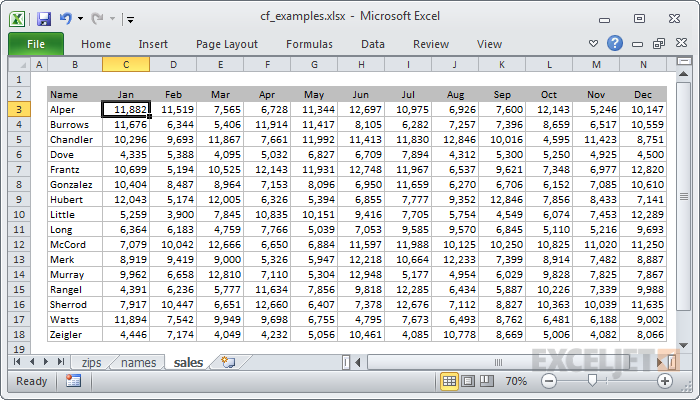
It’s nice to have all the information in one place, but you’d like to quickly see the 5 top and 5 bottom sales numbers, so you know where to focus your attention.
By using two built-in conditional formatting rules:

You can flag the top 5 values in green, and the bottom 5 values in red:

Want to learn more? See our video course on conditional formatting .
Highlighting values based on a variable input
Although Excel contains a large number of Conditional Formatting presets, the real power of Conditional Formatting comes from using formulas. Formulas allow you to create more powerful and flexible rules.
For example, suppose you want to explore a data set and highlight values above a certain value, in this case, 800?

By creating an input cell and referring to that input cell in a formula, you can make the threshold a variable.
<img loading=“lazy” src=“https://exceljet.net/sites/default/files/images/articles/inline/variable2.png" onerror=“this.onerror=null;this.src=‘https://blogger.googleusercontent.com/img/a/AVvXsEhe7F7TRXHtjiKvHb5vS7DmnxvpHiDyoYyYvm1nHB3Qp2_w3BnM6A2eq4v7FYxCC9bfZt3a9vIMtAYEKUiaDQbHMg-ViyGmRIj39MLp0bGFfgfYw1Dc9q_H-T0wiTm3l0Uq42dETrN9eC8aGJ9_IORZsxST1AcLR7np1koOfcc7tnHa4S8Mwz_xD9d0=s16000';" alt=“CF formula compares values to named range “input” - 14”>
Here the rule highlights all values greater than 800:

Here we’ve changed the input to 900, highlighting fewer values:

By making the rule variable, you create a model that lets you interactively explore the data. This is a great way to add some professional polish to a worksheet, because people love things that respond instantly to their actions.
Highlight entire rows based on values in a column
There are many situations where you may want to highlight an entire row based on a value that appears in one column. To do this with conditional formatting, you’ll need to use a formula and then lock the column reference as needed.
For example, let’s say you want to highlight orders in this set of data that are over $100:

The formula locks the column reference to test only values in column E:

The result:

Highlight rows based on an input cell
Building on the previous examples, here we are highlighting rows based on the value in an input cell named “owner”.


Build a search box
Using the same basic idea in the last example, you can actually build a search box using conditional formatting that searches multiple columns at the same time. This is a nice alternative to filtering because no data is hidden.
Video: How to build a search box with conditional formatting
