Purpose
Return value
Syntax
=AVERAGE(number1,[number2],...)
- number1 - A number or cell reference that refers to numeric values.
- number2 - [optional] A number or cell reference that refers to numeric values.
Using the AVERAGE function
The AVERAGE function calculates the average of numbers provided as arguments . To calculate the average, Excel sums all numeric values and divides by the count of numeric values.
AVERAGE takes multiple arguments in the form number1 , number2 , number3 , etc. up to 255 total. Arguments can include numbers, cell references, ranges, arrays, and constants. Empty cells, and cells that contain text or logical values are ignored. However, zero (0) values are included. You can ignore zero (0) values with the AVERAGEIFS function , as explained below.
The AVERAGE function will ignore logical values and numbers entered as text. If you need to include these values in the average, see the AVERAGEA function .
If the values given to AVERAGE contain errors, AVERAGE returns an error. You can use the AGGREGATE function to ignore errors .
Basic usage
A typical way to use the AVERAGE function is to provide a range , as seen below. The formula in F3, copied down, is:
=AVERAGE(C3:E3)

At each new row, AVERAGE calculates an average of the quiz scores for each person.
Blank cells
The AVERAGE function automatically ignores blank cells. In the screen below, notice cell C4 is empty, and AVERAGE simply ignores it and computes an average with B4 and D4 only:

However, note the zero (0) value in C5 is included in the average, since it is a valid numeric value. To exclude zero values, use AVERAGEIF or AVERAGEIFS instead. In the example below, AVERAGEIF is used to exclude zero values. Like the AVERAGE function, AVERAGEIF automatically excludes empty cells.
=AVERAGEIF(B3:D3,">0") // exclude zero

Mixed arguments
The numbers provided to AVERAGE can be a mix of references and constants:

=AVERAGE(A1,A2,4) // returns 3
Average with criteria
To calculate an average with criteria, use AVERAGEIF or AVERAGEIFS . In the example below, AVERAGEIFS is used to calculate the average score for Red and Blue groups:

=AVERAGEIFS(C5:C14,D5:D14,"red") // red average
=AVERAGEIFS(C5:C14,D5:D14,"blue") // blue average
The AVERAGEIFS function can also apply multiple criteria .
Average top 3
By combining the AVERAGE function with the LARGE function , you can calculate an average of top n values. In the example below, the formula in column I computes an average of the top 3 quiz scores in each row:

Detailed explanation here .
Weighted average
To calculate a weighted average, you’ll want to use the SUMPRODUCT function, as shown below:
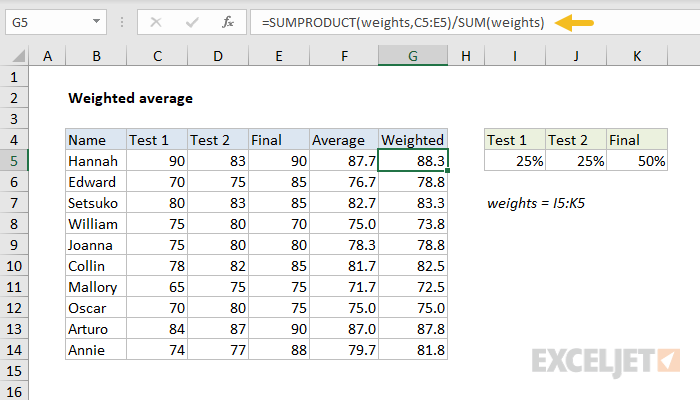
Read a complete explanation here .
Average without #DIV/0!
The average function automatically ignores empty cells in a set of data. However, if the range contains no numeric values, AVERAGE will return a #DIV/0! error. To avoid this problem, you can check the count of values with the COUNT function and the IF function like this:
=IF(COUNT(range)>0,AVERAGE(range),"") // check count first
When the count of numeric values is zero, IF returns an empty string (""). When the count is greater than zero, AVERAGE returns the average. This example explains this idea in more detail.
Manual average
To calculate the average, AVERAGE sums all numeric values and divides by the count of numeric values. This behavior can be replicated with the SUM and COUNT functions manually like this:
=SUM(range)/COUNT(range) // manual average calculation
Notes
- AVERAGE automatically ignores empty cells and cells with text values.
- AVERAGE includes zero values. Use AVERAGEIF or AVERAGEIFS to ignore zero values .
- Arguments can be supplied as constants, ranges, named ranges , or cell references.
- AVERAGE can handle up to 255 total arguments.
- To see a quick average without a formula , you can use the status bar .
Purpose
Return value
Syntax
=AVERAGEA(value1,[value2],...)
- value1 - A value or reference to a value that can be evaluated as a number.
- value2 - [optional] A value or reference to a value that can be evaluated as a number.
Using the AVERAGEA function
The AVERAGEA function returns the average of a set of supplied values. AVERAGEA will include the logical values TRUE and FALSE, and numbers represented as text in the calculation. The AVERAGE function ignores these values during calculation
AVERAGEA takes multiple arguments in the form of value1, value2, value3 , etc. up to 255 total. Arguments can include numbers, cell references, ranges, arrays, and constants. Empty cells are ignored, but zero (0) values are included.
Examples
To average values in the range A1:A10, including logical the logical values TRUE (1) and FALSE (0) and numbers entered as text, use AVERAGEA like this:
=AVERAGEA(A1:A10) // average numbers, logicals, numbers as text
One confusing aspect of the AVERAGE function compared to the AVERAGEA function is that both functions will evaluate logicals and numbers entered as text when they are hardcoded as constants in a formula :
=AVERAGE(TRUE,2) // returns 1.5
=AVERAGEA(TRUE,2) // returns 1.5
=AVERAGE("3",2) // returns 2.5
=AVERAGEA("3",2) // returns 2.5
However, the AVERAGE function will ignore logicals or numbers entered as text when they appear in cell references . You can see this behavior in the worksheet example shown above.
Notes
- Values can be supplied as numbers, ranges, named ranges, or cell references that contain values. Up to 255 arguments can be supplied.
- To calculate the average, Excel adds the numeric value of each value together and divides by the total number of values supplied.
- AVERAGEA evaluates TRUE as 1 and FALSE as zero.
