Purpose
Return value
Syntax
=BINOMDIST(number_s,trials,probability_s,cumulative)
- number_s - The number of successes.
- trials - The number of independent trials.
- probability_s - The probability of success on each trial.
- cumulative - TRUE = cumulative distribution function, FALSE=probability mass function.
Using the BINOMDIST function
The BINOMDIST function returns the individual term binomial distribution probability. You can use BINOMDIST to calculate probabilities that an event will occur a certain number of times in a given number of trials. BINOMDIST returns probability as a decimal number between 0 and 1.
Binary data occurs when an observation can be placed into only two categories. For example, when tossing a coin, the result can only be heads or tails. Or, when rolling a die, the result can either be 6 or not 6.
Note: the BINOMDIST function is classified as a compatibility function , replaced by the BINOM.DIST function .
Example
In the example shown, the BINOMDIST function is used to calculate the probability of rolling a 6 with a die. Since a die has six sides, the probability of rolling a 6 is 1/6, or 0.1667. Column B holds the number of trials, and the formula in C5, copied down, is:
=BINOMDIST(B5,10,0.1667,TRUE) // returns 0.1614
which returns the probability of rolling zero 6s in 10 trials, about 16%. The probability of rolling one 6 in 10 trials is about 32%.
The formula in D5 is the same, except the cumulative argument has been set to TRUE. This causes BINOMDIST to calculate the probability that there are “at most” X successes in a given number of trials. The formula in D5, copied down, is:
=BINOMDIST(B5,10,0.1667,TRUE) // returns 0.1614
In cell D5, the result is the same as C5 because the probability of rolling at most zero 6s is the same as the probability of rolling zero 6s. In cell D8, the result is 0.9302, which means the probability of rolling at most three 6s in 10 rolls is about 93%.
Notes
- BINOMDIST returns probability as a decimal number between 0 and 1.
- Number_s should be an integer, and will be truncated to an integer if not.
- Trials should be an integer, and will be truncated to an integer if not.
- If number_s, trials, or probability_s are not numbers, BINOMDIST returns a #VALUE! error.
- If number_s < 0 or number_s > trials, BINOMDIST returns a #NUM! error.
- If probability_s < 0 or probability_s > 1, BINOMDIST returns a #NUM! error value.
Purpose
Return value
Syntax
=CORREL(array1,array2)
- array1 - The first set of data values.
- array2 - The second set of data values.
Using the CORREL function
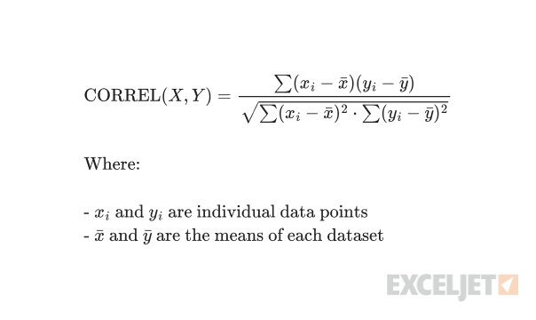
The CORREL function calculates the Pearson correlation coefficient between two data sets. It measures both the strength and direction of the linear relationship between variables, providing a standardized measure that ranges from -1 to 1.
Key features
- Returns values between -1 and 1 (inclusive)
- Positive values close to 1 indicate positive correlation
- Negative values close to -1 indicate negative correlation
- Values close to zero indicate weak correlation
- Unit-independent and standardized measure
- Both arrays must have the same number of data points
- Works with numbers only - text and logical values are ignored
Note: Excel also provides PEARSON function which is identical to CORREL. Both calculate the Pearson product-moment correlation coefficient.
- Example #1 - Strong Positive Correlation
- Example #2 - Strong Negative Correlation
- Example #3 - Weak Correlation
- When to use CORREL
- Formula Definition
- Notes
Example #1 - Strong Positive Correlation
In this example, we’ll examine the relationship between temperature (°F) and ice cream sales ($). As temperature increases, ice cream sales tend to increase as well, demonstrating a strong positive correlation.
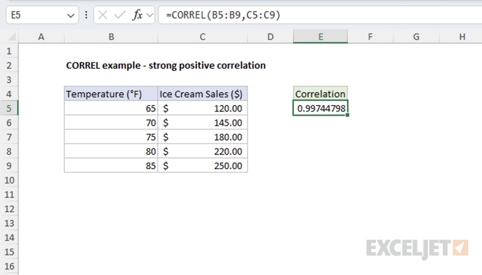
=CORREL(B5:B9,C5:C9) // returns 0.997447985
The result indicates a strong positive correlation between temperature and ice cream sales.
Example #2 - Strong Negative Correlation
Here we examine the relationship between a car’s mileage (miles) and its resale value. As mileage increases, the car’s value decreases proportionally, showing a strong negative correlation.
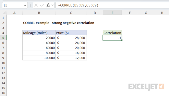
=CORREL(B5:B9,C5:C9) // returns -1
The result confirms a strong negative correlation between car mileage and its market value.
Example #3 - Weak Correlation
This example illustrates two variables with a weak relationship: daily temperature and coffee sales. While there might be some relationship, it’s not very strong.
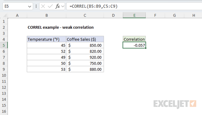
=CORREL(B5:B9,C5:C9) // returns -0.057
The result close to zero indicates a weak negative correlation between temperature and coffee sales.
When to use CORREL
Use CORREL when you need to quantify the linear relationship between two sets of numerical data in Excel. Choose CORREL over COVARIANCE.P or COVARIANCE.S (covariance functions) when you want a standardized measure that’s easy to interpret regardless of the units involved. Use the covariance functions when you care about the magnitude of change in addition to the direction and strength of the relationship between variables.
Key advantages
- Standardized scale (-1 to +1) makes interpretation easier
- Unit-independent - can compare relationships across different measurement scales
- Provides both direction and strength of relationship
- Widely recognized and understood statistical measure
Formula definition
Notes
- Both arrays must contain the same number of values
- Empty cells, text, and logical values are ignored
- Returns #DIV/0! error if either array has zero variance (all values are identical)
- Returns #N/A error if arrays have different lengths
- Only measures linear relationships - may miss non-linear associations
