Explanation
In this example, the goal is to create a list of pay dates that follow a biweekly schedule. A biweekly pay schedule means employees are paid every two weeks on a given day of the week. Each pay period is 14 days, and there are usually 26 pay dates per year, though occasionally 27 depending on the calendar. In the worksheet shown above, pay dates are every other Friday, beginning on the first Friday of the year. We can solve this problem with the SEQUENCE function, as explained below.
Background study
If you are unfamiliar with the SEQUENCE function, or dynamic array formulas in general, these links will help you get up to speed quickly:
- How to use the SEQUENCE function - overview
- The SEQUENCE function - 3 min video
- SEQUENCE of dates - 3 min video
- Dynamic Array Formulas - video training
SEQUENCE function
The SEQUENCE function is used to generate numeric sequences with the following syntax:
=SEQUENCE(rows,[columns],[start],[step])
- rows - the number of rows to return
- columns - the number of columns to return
- start - the starting value
- step - the increment to use between values
In this example, the goal is to generate a sequence of 26 pay dates, each 14 days apart. To generate the dates, the formula in cell D5 is:
=SEQUENCE(B8,1,B5,14)
Inside SEQUENCE, we provide the following values:
- rows - B8 (26)
- columns - 1
- start - B5 (January 6, 2023 = 44932)
- step - 14 (days between dates)
We can use SEQUENCE to generate dates in Excel because Excel dates are just large serial numbers . The serial number for January 1, 2023, is 44927, so the serial number for January 6, 2023, is 44932. The formula is evaluated by Excel’s formula engine like this:
=SEQUENCE(B8,1,B5,14)
=SEQUENCE(26,1,44932,14)
Essentially, we are asking SEQUENCE for 26 numbers that start on 44927 and are incremented by 14. With the above configuration, SEQUENCE returns an array that contains 26 dates in serial number format:
{44932;44946;44960;44974;44988;45002;45016;45030;45044;45058;45072;45086;45100;45114;45128;45142;45156;45170;45184;45198;45212;45226;45240;45254;45268;45282}
These values spill into the range D5:D30. When properly formatted, they display as dates. In this particular example, we are using the custom number format below:
ddd d-mmm-yyyy
This causes Excel to display an abbreviated day name (i.e. “Fri”) before the date to make it easy to verify correct results.
Holidays
The formula above does not take into account pay dates that land on holidays, which are typically moved to the previous business day. One way to do this is to add in the WORKDAY function , which can calculate the next or previous workday from a given start date, taking into account weekends and holidays. The generic formula looks like this:
=WORKDAY(SEQUENCE(n,1,start,14)+1,-1,holidays)
Where n is the number of dates to generate, and holidays is a range or array that contains dates that are holidays. The worksheet below shows how this formula can be adapted to the worksheet discussed above:
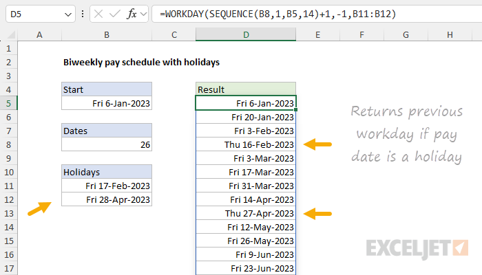
Here, we basically feed the results from SEQUENCE directly into the WORKDAY function, with the range B11:B12 given for the holidays argument. We have to use a bit of trickery here to get WORKDAY to check the date returned by SEQUENCE. We do this by asking WORKDAY for the workday previous to the date + 1. In other words, we add 1 to the date, then ask WORKDAY for the previous workday by providing -1 for days. This causes WORKDAY to check the original date from SEQUENCE, and step back to the previous workday if the pay date is in fact a holiday. With the (arbitrary) dates of Feb 17, 2023, and April 28, 2023, provided as holidays in the range B11:B12, notice how the formula rolls back to Thursday in cells D8 and D13.
Explanation
In this example, we’ll use SEQUENCE to generate all dates in a given month. Creating a complete list of dates for a specific month is a common Excel task with many practical applications, from building project timelines and work schedules to generating calendar views and tracking daily data. The input is any date within the target month (it doesn’t matter which specific day), and the output is a dynamic list that automatically adjusts when you change the input date. The technique works because Excel stores dates as serial numbers , allowing SEQUENCE to count through them just like any other numeric sequence. Although the core of the solution is SEQUENCE, it’s also interesting how we use the DAY and EOMONTH functions to calculate the inputs to SEQUENCE. The EOMONTH function is particularly useful and comes up in all kinds of other formulas. The DAY function (together with EOMONTH) is a clever way to get the total days in a month.
- The SEQUENCE function
- SEQUENCE with dates
- SEQUENCE to list all dates in a month
- LET version of the formula
- All dates between two dates
- Current month dates with TODAY function
- Approach for older versions of Excel
- Useful links
The SEQUENCE function
The SEQUENCE function can generate numeric sequences using a generic syntax like this:
=SEQUENCE(rows,[columns],[start],[step])
Rows is the number of rows to return, columns is the number of columns to return, start is the starting value, and step is the increment to use between values. The arguments columns , step , and start all default to 1. For example, we can ask for the numbers 1-10 like this:
=SEQUENCE(10) // returns {1;2;3;4;5;6;7;8;9;10}
To get the numbers 51-60, we can set start to 50:
=SEQUENCE(10,,50) // returns {50;51;52;53;54;55;56;57;58;59}
In both formulas above, SEQUENCE generates an array of numbers that will spill into 10 rows.
SEQUENCE with dates
Because dates are just numbers in Excel, we can easily configure SEQUENCE to output dates. For example, to output the first 5 days in May 2025, we could use a formula like this:
=SEQUENCE(5,,"1-May-2025") // returns {45778;45779;45780;45781;45782}
The result will be an array of serial numbers, as shown above. In this array, the number 45778 corresponds to the date 1-May-2025 in Excel’s date system . To display these numbers as dates, apply number formatting .
SEQUENCE to list all dates in a month
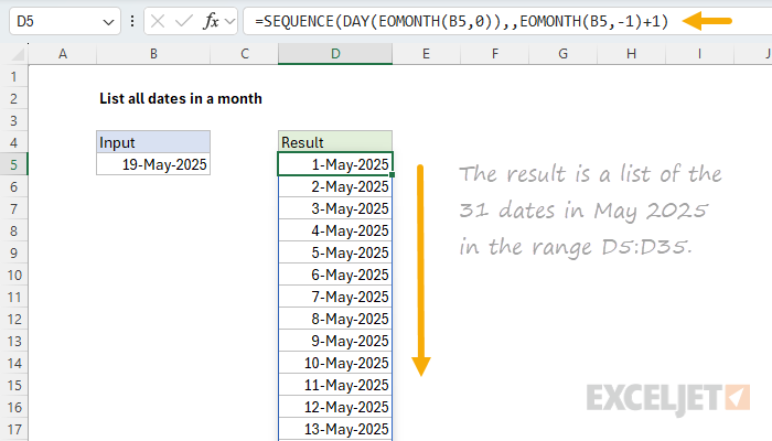
In the worksheet shown, we want to generate a list of all dates in a given month, where the month is input as a date in cell B5. To use SEQUENCE for this task, we need to calculate two input values based on the date in B5: (1) the number of days in the month and (2) the first day of the month. To get the number of days in the month, we can use the DAY function like this:
=DAY(EOMONTH(B5,0))
In this snippet, we use EOMONTH to get the last day of the current month (note the offset is zero), then we use the DAY function to get the number of days in the month. For example, with a date like 15-May-2025 in B5, EOMONTH returns the date 31-May-2025, and DAY returns 31, which is equal to the number of days in the month. To get the first day of the month, we can use the EOMONTH function like this:
=EOMONTH(B5,-1)+1 // get first day in month
Here, we use EOMONTH to travel back to the last day of the “previous” month and then add 1 to move forward one day to land on the first day of the “current” month, relative to the date in B5. The final formula in cell D5 looks like this:
=SEQUENCE(DAY(EOMONTH(B5,0)),,EOMONTH(B5,-1)+1)
The inputs provided to SEQUENCE are as follows:
- rows - DAY(EOMONTH(B5,0)) // days in month
- columns - omitted, defaults to 1
- start - EOMONTH(B5,-1)+1 // first of month
- step - omitted, defaults to 1
With the above configuration, SEQUENCE returns an array of 31 serial numbers that correspond to all dates in May 2025:
{45778;45779;45780;45781;45782;45783;45784;45785;45786;45787;45788;45789;45790;45791;45792;45793;45794;45795;45796;45797;45798;45799;45800;45801;45802;45803;45804;45805;45806;45807;45808}
You must apply a number format for dates to display these serial numbers as dates.
The output is fully dynamic. If the date in B5 is changed to 9-Jun-2025, the formula will list the 30 dates in June 2025. Notice that the actual date given to SEQUENCE doesn’t matter because the formula automatically calculates the first day of the month (with EOMONTH, as explained above) for the start value in SEQUENCE.
LET version of the formula
We can use the LET function to clean up the formula above somewhat like this:
=LET(
  date,B5,
  first,EOMONTH(date,-1)+1,
  days,DAY(EOMONTH(date,0)),
  SEQUENCE(days,,first)
)
This is an excellent example of how the LET function creates cleaner code and results in a formula that is easier to read and debug.
Tip: To see the entire formula above in the formula bar, use the shortcut Control + U.
All dates between two dates
The generic formula to create a list of all dates between two dates looks like this:
=SEQUENCE(end-start+1,1,start)
This can be adapted to generate a list of all dates in a month like this:
=LET(
  date,B5,
  first,EOMONTH(date,-1)+1,
  last,EOMONTH(date,0),
  SEQUENCE(last-first+1,,first)
)
The results will be the same, but I think the first formula above is slightly easier to understand and configure.
Current month dates with TODAY function
To generate a list of all dates in the current month (without needing to specify a date in a cell), you can replace the cell reference with the TODAY function :
=SEQUENCE(DAY(EOMONTH(TODAY(),0)),,EOMONTH(TODAY(),-1)+1)
This formula automatically lists all dates for the current month and updates continuously. For example, if today is June 15, 2025, the formula will generate all 30 dates in June 2025. Tomorrow, if it’s still June, it will show the same list, but if the month changes to July, it will automatically update to show all 31 dates in July 2025.
The formula works exactly the same way as the previous version, but uses TODAY() instead of a cell reference to determine the target month. This approach is useful for things that need to stay up-to-date:
- Dashboard reports that always show current month data
- Daily logs or tracking sheets that auto-update
- Templates that need to work regardless of when they’re opened
Approach for older versions of Excel
In older versions of Excel, we don’t have the SEQUENCE function, so we need to take a different approach. There are many options for this kind of problem, but I think the approach shown below works pretty well:
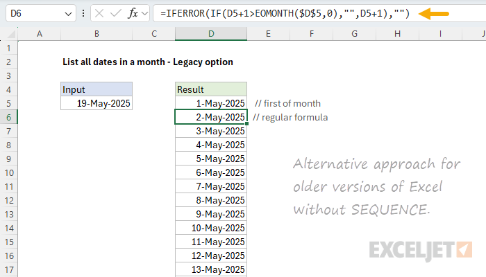
There are two different formulas in the worksheet. The first formula in cell D5 gets the first-of-month from the date in cell B5 like this:
=EOMONTH(B5,-1)+1
The second formula, entered in cell D6 and copied down manually until it returns nothing, looks like this:
=IFERROR(IF(D5+1>EOMONTH($D$5,0),"",D5+1),"")
Working from the inside out, the core formula increments dates with the IF function like this:
IF(D5+1>EOMONTH($D$5,0),"",D5+1)
The formula first adds 1 to the value in D5, then checks if the resulting date is greater than the last day of the month, calculated with EOMONTH($D$5,0) . If so, IF returns an empty string (""), which looks like a blank cell. If not, the result is D5+1, which adds one day to the previous date. As the formula is copied down, it generates all dates in the given month and then begins to output “blank” cells. To handle the #VALUE! error that arises after the first blank cell, the core formula above is wrapped in the IFERROR function :
=IFERROR(formula,"")
IFERROR catches the value error and returns an empty string ("") when necessary. The result is that you can copy the formula well past the end of the month and not see any errors.
Useful links
- How to use the SEQUENCE function - overview
- The SEQUENCE function - 3 min video
- SEQUENCE of dates - 3 min video
- Dynamic Array Formulas - Video training
