Purpose
Return value
Syntax
=BYROW(array,function)
- array - The array or array to process.
- function - The function to apply to each row.
Using the BYROW function
The Excel BYROW function applies a function to each row in array and returns one result per row in a single array . The purpose of BYROW is to process data in an array or range in a “by row” fashion. For example, if BYROW is given an array with 10 rows, BYROW will return an array with 10 results. The calculation performed on each row can be a stock function like SUM, COUNT, etc., or a custom LAMBDA function designed to operate on row values. BYROW can accept an abbreviated “eta lamba” syntax for simple operations like SUM, as explained below.
The concept and syntax
Essentially, BYROW allows you to loop over all rows in a range or array and perform a custom calculation on each row in a single formula. The second argument, function, determines the calculation performed :
=BYROW(array,function)
The function can be provided in two ways: a short-form “eta lambda” syntax or a long-form custom LAMBDA syntax. For example, to sum each row in an array, the short-form syntax looks like this:
=BYROW(array,SUM)
The long-form custom syntax looks like this:
=BYROW(array,LAMBDA(row,SUM(row))
Why two syntax options? The short form is for convenience. It is concise and easy to read. However, the behavior cannot be customized. The long-form syntax uses the LAMBDA function and can be customized as desired. See below for an example of BYROW formulas that use both options.
Note: in the examples above, we use the variable name “row” in the LAMBDA function for clarity. However, you are free to use whatever name you like.
Example - sum all rows
In the worksheet below, the BYROW function is used to sum the values in each row of the range C5:H15. The formula in cell J5 looks like this:
=BYROW(C5:H15,LAMBDA(row,SUM(row)))

The BYROW function returns all results at once in a single array. Because there are 11 rows in data, the result is an array that contains 11 sums like this:
{432;440;403;455;479;433;426;463;407;431;519}
The values in this array spill into the range J5:J15. The formulas below are other examples of how BYROW can be used on the same data with formulas that follow the same pattern:
=BYROW(data,LAMBDA(row,MAX(row))) // max
=BYROW(data,LAMBDA(row,MIN(row))) // min
=BYROW(data,LAMBDA(row,AVERAGE(row))) // average
Example - Short form “eta lambda” syntax
While BYROW is designed to accept a function defined by LAMBDA, it will also accept a short-form “eta lambda” syntax for simple operations. Using the eta lambda syntax, you can pass a function by name only into BYROW like this:
=BYROW(array,SUM)
This formula is equivalent to the long-form version:
=BYROW(array,LAMBDA(x,SUM(x)))
For example, in the worksheet below, we have adapted the formula in J5 to use the short-form syntax. The formula now looks like this:
=BYROW(C5:H15,SUM)

The Excel formula engine knows how to pass each row into the SUM function, and the results are exactly the same as the long-form version. You can use the same syntax to call other functions like this:
=BYROW(array,SUM) // sum each row
=BYROW(array,MAX) // max of each row
=BYROW(array,MIN) // min of each row
=BYROW(array,COUNT) // count of each row
The short-form eta syntax works for functions that accept a single argument, such as SUM, AVERAGE, MIN, MAX, COUNT, COUNTA, etc. It will not work in all scenarios because the logic can’t be modified. For example, the formula in the next section below can’t use the eta lambda syntax.
Example - Count cells over 90
In this example, the goal is to count the values in each row greater than 90. The formula is a bit more complex because we need more logic. This is a situation where we can’t use the short-form syntax. The formula in cell K5 looks like this:
=BYROW(C5:H15,LAMBDA(row,SUM(--(row>90))))

Working from the inside out, a custom lambda counts all values in a row greater than 90:
LAMBDA(row,SUM(--(row>90))) // custom lambda
The logical expression row>90 returns an array of TRUE and FALSE values, and we use a double negative (–) to coerce these values to 1s and 0s. The SUM function then sums the 1s and 0s, and the result is the count of values greater than 90:
SUM(--(row>90))
The LAMBDA runs on each row in the data. Since there are 11 rows in the range B5:H15, BYROW returns 11 results that spill into the range K5:K15. See Boolean operations in array formulas for more information about the logic inside of SUM.
You could use COUNTIFS instead of SUM to solve this problem. However, COUNTIFS requires a range , which means you can’t give BYROW an array if you use COUNTIFS in the calculation. For this reason, I generally avoid the *IFS functions when working with the new dynamic array functions where arrays are more common.
Example - BYROW with multiple functions
It is also possible to configure BYROW to run more than one function at the same time, although it is not obvious how. The trick is to wrap the functions in the HSTACK or VSTACK functions (depending on the layout needed). For example, in the worksheet below, BYROW is configured to return the sum, the maximum value, and the minimum value for each row at the same time. The formula in J5, copied down, is:
=BYROW(C5:H15,HSTACK(SUM,MAX,MIN))

Although this formula uses the short-form syntax, you can take the same approach with custom LAMBDA calculations.
Because of the current array of arrays limitation in Excel, this formula will not spill down across all rows. It will initially only calculate results for the first row. You will then need to copy the formula manually to all rows in a second step.
Purpose
Return value
Syntax
=CHOOSECOLS(array,col_num1,[col_num2],...)
- array - The array to extract columns from.
- col_num1 - The numeric index of the first column to return.
- col_num2 - [optional] The numeric index of the second column to return.
Using the CHOOSECOLS function
The Excel CHOOSECOLS function returns specific columns from an array or range . The columns to return are provided as numbers in separate arguments. Each number corresponds to the numeric index of a column in the source array. The result from CHOOSECOLS is always a single array that spills onto the worksheet.
The first argument in the CHOOSECOLS function is the array , which can be a range, an array constant, or an array generated by another formula. Additional arguments are in the form: col_num1 , col_num2 , col_num3 , etc., and should be the numeric index of the column to extract.
Basic usage
To get columns 1 and 3 from an array, you can use CHOOSECOLS like this:
=CHOOSECOLS(A1:C5,1,3) // columns 1 and 3
To get the same two columns in reverse order:
=CHOOSECOLS(A1:C5,3,1) // columns 3 and 1
CHOOSECOLS will return a #VALUE! error if a requested column number is out of range:
=CHOOSECOLS(A1:C5,4) // returns #VALUE!
With an array constant
Another option for specifying which columns to return is to use an array constant like {1,2,3} as the second argument ( col_num1) . In the example below, the formula in H3 is:
=CHOOSECOLS(B3:F9,{1,3,5})
With the array constant {1,3,5} given as the second argument, CHOOSECOLS returns columns 1, 3, and 5:

The array constant provided can be in the form {1,2,3} or {1;2;3}.
With negative column numbers
A nice feature of CHOOSECOLS is that you can use negative column numbers to extract columns from the end of a range. For example, to get the last column of a range, you can use a formula like this:
=CHOOSECOLS(range,-1)
To get the second-to-last column, you can use:
=CHOOSECOLS(range,-2)
To get the last three columns in the order that they appear:
=CHOOSECOLS(range,-3,-2,-1)
You can also mix negative and positive row numbers. To return the first and last columns at the same time:
=CHOOSECOLS(range,1,-1)
With arrays
As seen above, you can use an array constant as the second argument in CHOOSECOLS to specify columns. You can also use an array generated with a formula. For example, in the worksheet below, we use the SEQUENCE function inside CHOOSECOLS to reverse the column order of the range B3:D9 with a formula like this in cell F3:
=CHOOSECOLS(B3:D9,-SEQUENCE(COLUMNS(B3:D9)))
Since the range B3:D9 contains 3 columns, COLUMNS returns 3 and SEQUENCE returns {1;2;3}:
SEQUENCE(3) // returns {1;2;3}
The negative sign before SEQUENCE converts the array to {-1;-2;-3}:
-SEQUENCE(3) // returns {-1;-2;-3}
Simplifying, the final CHOOSECOLS formula looks like this:
=CHOOSECOLS(B3:D9,{-1;-2;-3})
The result is that CHOOSECOLS returns the 3 columns in B3:D9 in reverse order:
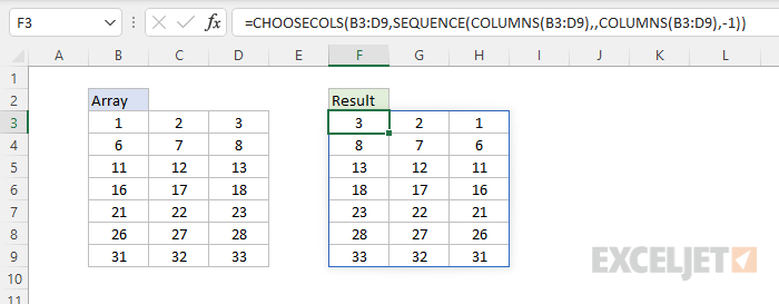
The CHOOSECOLS returns all columns in the array: the last column (-1), the second to last column (-2), and the third to last column (-3).
Notes
- CHOOSECOLS will return a #VALUE error if a column number is out of range.
