Explanation
In this example, the goal is to calculate a retirement date at age 60, based on a given birthdate. The simplest way to do this is with the EDATE function. The EDATE function will return a date n months in the future or past when given a date and the number of months to traverse. In this case, we want a date 60 years from the birthdate in column C, so the formula in D5 is:
=EDATE(C5,12*60) // 60 years from birthdate
The date comes from column C. For months , we need the equivalent of 60 years in months. Since most people don’t know how many months are in 60 years, a nice way to do this is to embed the calculation in the formula like this:
12*60 // 720 months = 60 years
Inside the EDATE function, Excel will perform the math and return 720 directly to EDATE as the months argument . Embedding calculations this way can help make the assumptions and purpose of a formula easier to understand. To use a retirement age of 65, just adjust the calculation:
12*65 // 780 months = 65 years
In cell D5, returns the date March 10, 2023. As the formula is copied down column D, a different date is returned for each person in the list based on their birthdate.
Note: EDATE returns a date as a serial number , so apply a date number format to display as a date.
End of month
To calculate a retirement date that lands at the end of the month, you can use the EOMONTH function instead of the EDATE function like this:
=EOMONTH(C5,12*60) // +60 years at end of month
EOMONTH works like EDATE, but always returns the end of the month. If there is a rule that people with birthdays that fall on the first of the month retire on the last day of the previous month, the formula can be adjusted like this:
=EOMONTH(C5,(12*60)-(DAY(C5)=1))
Here, the logical expression DAY(C5)=1 is subtracted from 12*60 = 720. The DAY function returns the day of the birthdate. If the day is 1, the expression returns TRUE. Otherwise, the expression returns FALSE. The math operation of subtraction coerces TRUE to 1 and FALSE to zero. The result is that EOMONTH moves forward 719 months if a birthday falls on the first of the month, and 720 months if not. This moves first-of-month birthdays to the last day of the previous month.
Year only
To return the retirement year only, we can nest EDATE inside the YEAR function like this:
=YEAR(EDATE(C5,12*60)) // return year only
Since we already have the date in column D, the formula in column E is:
=YEAR(D5) // year from date in D5
The YEAR function returns the year of the date returned by EDATE.
Years remaining
In column F, we calculate the years remaining with the YEARFRAC function like this:
=YEARFRAC(TODAY(),D5)
This formula returns the difference between today’s date and the calculated retirement date in column D. As the retirement date approaches, the years remaining will automatically decrease. To guard against a retirement date that has already passed, the formula in column F uses the SIGN function to change the years remaining to a negative number like this:
=YEARFRAC(TODAY(),D5)*SIGN(D5-TODAY()) // make negative if past
The SIGN function simply returns the sign of a number as 1, -1, or 0. To use it, we subtract today’s date from the retirement date. If the result is positive, the retirement date is in the future and SIGN returns 1, which does not affect the result from YEARFRAC. If the result is negative, the retirement date is in the past and SIGN returns -1, flipping the YEARFRAC calculation to a negative number. You can see the result in row 8, where the retirement date has already passed.
Other uses
This same approach can be used to calculate dates for a wide variety of use cases:
- Warranty expiration dates
- Membership expiration dates
- Promotional period end date
- Shelf life expiration
- Inspection dates
- Certification expiration
Explanation
In this example, the goal is to calculate the time remaining before an expiration date. There are many ways to do something like this in Excel, and in this article, we’ll look at three different approaches:
- Calculating the remaining time in days
- Calculating the remaining time in years, months, and days
- Calculating the percentage of shelf life remaining.
Each approach includes an explanation of how the formula works.
Important notes
- Examples use the named range “cdate”, which points to a cell that contains the “current date”. This makes it easy to change the date used to calculate the remaining time. This also makes it possible to calculate results based on a future date. For example, you can easily change the date to the first of next month to evaluate expiration dates as of that date.
- If you prefer, you can replace the hardcoded date in cdate with the TODAY function , so that it always contains the current date. However, be aware that over time more and more items will appear as expired in this particular example.
- You should be familiar with the concept of concatenation in Excel , the process of joining values together in text strings.
How Excel Tracks Time
Excel tracks time using its date system, which is based on serial numbers . Each date is represented as a unique serial number, where January 1, 1900, is serial number 1, January 2, 1900, is serial number 2, and so on. This system allows you to perform date arithmetic easily in Excel. For example, subtracting one date from another yields the number of days between the two dates. Understanding this date system is important for creating and working with date-related formulas in Excel.
Approach 1: Calculating Time in Days
The simplest approach is to calculate the remaining time in days , which takes advantage of Excel’s built-in date system and requires no special date functions. In the worksheet below, the formula in cell E5 is:
=IF(C5>cdate,C5-cdate&" days","Expired")
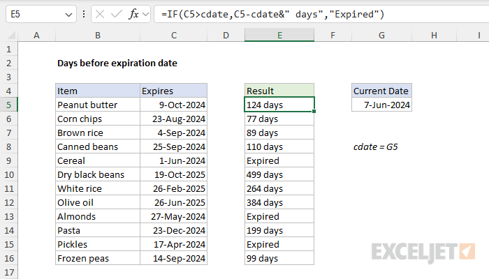
The logic of the formula works as follows. At a high level, the IF function controls the flow of the formula. Inside IF, the logical test is configured to check if the expiration date (C5) is greater than the current date ( cdate ):
=IF(C5>cdate,
Excel dates are just serial numbers underneath, so if the expiration date in C5 is larger than the “current” date (cdate) it means the date is still in the future. The logical test will return TRUE and the formula will subtract cdate from C5 and concatenate “days " to the result:
=IF(C5>cdate,C5-cdate&" days",
Otherwise, the expiration date in C5 is not larger than the current date, which means the expiration has already been reached. In that case, the logical test will return FALSE and the IF function will return “Expired” as a result.
Approach 2: Calculating Time in Years, Months, and Days
Another approach is to calculate the time remaining in years, months, and days. This requires a more elaborate formula based on the DATEDIF function. In the worksheet below, the formula in cell E5, with line breaks* added for readability, looks like this:
=IF(C5>cdate,
DATEDIF(cdate,C5,"y")&" years, "&
DATEDIF(cdate,C5,"ym")&" months, " &
DATEDIF(cdate,C5,"md")&" days",
"Expired")
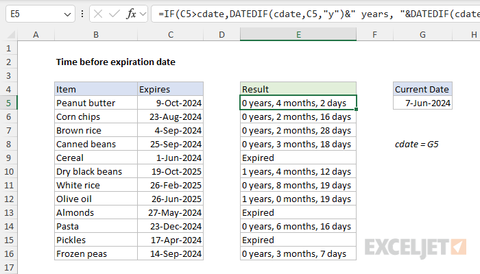
Here, we calculate the time remaining before the expiration date in a combination of years, months, and days all concatenated together in a text string. The tricky part of the problem is that we need to ensure we are correctly “backing out” the time units we have already accounted for. Luckily, the DATEDIF function is designed just for this purpose.
At the top level, this formula again uses the IF function to control flow by first testing the expiration date to ensure it is still in the future. If so, we calculate a final result with three separate calls to DATEDIF. If not, we simply return “Expired”:
=IF(C5>cdate,...,"Expired")
When the expiration date is greater than the current date, we call DATEDIF three times like this:
DATEDIF(cdate,C5,"y")&" years, "&
DATEDIF(cdate,C5,"ym")&" months, " &
DATEDIF(cdate,C5,"md")&" days",
- DATEDIF(cdate,C5,“y”) - Calculate the number of complete years between the current date and the expiration date.
- DATEDIF(cdate,C5,“ym”) - Calculate the number of complete months, ignoring the years.
- DATEDIF(cdate,C5,“md”) - Calculate the number of days, ignoring the years and months.
The three results are then concatenated into a single text string, which IF returns as the final result. See this page for a more detailed example of this approach, including a simplified formula based on the LET function .
*You can add line breaks to a formula in Excel with the Keyboard Shortcut Alt + Enter.
Approach 3: Calculating Percentage of Shelf Life Remaining
In this last approach, we calculate the percentage of the shelf life that remains. Note that this requires us to have a “Packed” or “Manufactured” date to calculate the product’s total shelf life. In the worksheet below, the formula in cell F5, copied down, is:
=(D5-cdate)/(D5-C5)
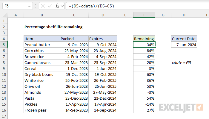
One key difference between this formula and the two previous formulas is that we are not using the IF function to control flow. Instead, we are simply calculating a percentage and allowing negative percentage results to pass through. The formula used in the worksheet is:
=(D5-cdate)/(D5-C5)
- (D5-cdate) - Calculate the time to expiration in days, by subtracting the current date (cdate) from the packed date (D5).
- (D5-C5) - Calculate the total shelf life in days, by subtracting packed date (C5) from the expiration date (D5).
- Divide time to expiration in days by total shelf life in days
The result is a number like 0.338 that must be then formatted as a percentage .
Creating an expiration date
To create an expiration date based on a given date you can simply add the number of days until expiration. With a date in A1:
=A1+30 // 30 days in the future
=A1+90 // 90 days in the future
Alternatively, you can use the EDATE function to calculate in months:
=EDATE(A1,1) // 1 month in the future
=EDATE(A1,3)  // 3 months in the future
Both options above will work fine, but one advantage of EDATE is that it will preserve the day from the original date in A1.
Explanation
Working from the inside out, EDATE first calculates a date 6 months in the future. In the example shown, that date is December 24, 2015.
Next, the formula subtracts 1 day to get December 23, 2015, and the result goes into the WORKDAY function as the start date, with days = 1, and the range B9:B11 provided for holidays.
WORKDAY then calculates the next business day one day in the future, taking into account holidays and weekends.
If you need more flexibility with weekends, you can use WORKDAY.INTL.
Explanation
Working from the inside out, we use the DATEDIF function to calculate how many complete years are between the original anniversary date and the “as of” date, where the as of date is any date after the anniversary date:
DATEDIF(B5,C5,"y")
Note: in this case, we are arbitrarily fixing the “as of” date as June 1, 2017 in all examples.
Because we are interested in the next anniversary date, we add 1 to the DATEDIF result, then multiply by 12 to convert to years to months.
Next, the month value goes into the EDATE function, with the original date from column B. The EDATE function rolls the original date forward by the number of months given in the previous step which creates the next upcoming anniversary date.
As of today
To calculate the next anniversary as of today, use the TODAY() function for the “as of” date:
=EDATE(date,(DATEDIF(date,TODAY(),"y")+1)*12)
