Can Pivot Tables Save Your Job?

Overview | Why Pivot? | Story | Examples

This article is for those of you who don’t get pivot tables. Maybe you tried pivot tables once, and didn’t see what the big deal was, or maybe you got frustrated when a pivot table wouldn’t behave. They can be that way.

I’m not going to mince words. If you use Excel on a regular basis, you need to know how to use pivot tables. Period. I’ll get to some good reasons below, but first, a quick story.

When I first learned pivot tables in the late 1990s, I was working as a manager for a medium sized (US $50M) company in the translation industry that was going through a major restructuring. My boss, who had hired me 3 months earlier, had done his part in the restructuring, personally laying off about 30 people one dark week in November. A big wig from Singapore was in town, and they actually sat together in the main conference room and called people up over the PA system. It was brutal. All week, people filed past my office to the conference room, and came back stunned and upset, many in tears.

At the end of the week, the company repaid my boss for handling that miserable job by laying him off too. You gotta love corporate America.

Looking for good tips? See 23 things you should know about pivot tables .

What’s this got to do with pivot tables?

Yes, let’s get to that. The upshot of my boss being suddenly sacked was that I was “promoted” to a new role, running an office with about $10M of annual revenue running through it, with less than half the original staff, most of whom were now supposed to play different roles in the company (with no job descriptions, naturally). The remaining staff were not, as you might expect, completely trusting of the company at that point. Beyond ordinary chaos, there was a deep current of fear running through the office. People thought it was just a matter of time before the axe dropped on them.

More on that in a minute…

In the meantime, of course, there was work to do. We had sales people selling new jobs, we were just starting the largest project we’d ever tackled: a 25-language job for a large computer company with a budget well over $1M. And we had lots of jobs already in progress.

As the manager, I was responsible for submitting sales forecasts, recognizing revenue on existing projects, estimating invoicing, knowing what jobs were won and lost, knowing who my top customers were, and making sure existing projects came out ok.

We had no integrated systems of any kind. No CRM system, no way to forecast sales, no project tracking app, nothing.

Luckily, I had my trusty Toshiba laptop (a brick, but running NT, thankfully, not Windows 95), and I had just discovered pivot tables. After a few very frustrating early weeks (pivot tables were quite delicate at the time and fell apart at the slightest provocation), I realized that if I could just get together the right data, I could use pivot tables to generate any report I needed for myself or my management. And, a few months later, that’s just what I did.

Pivot tables give you answers

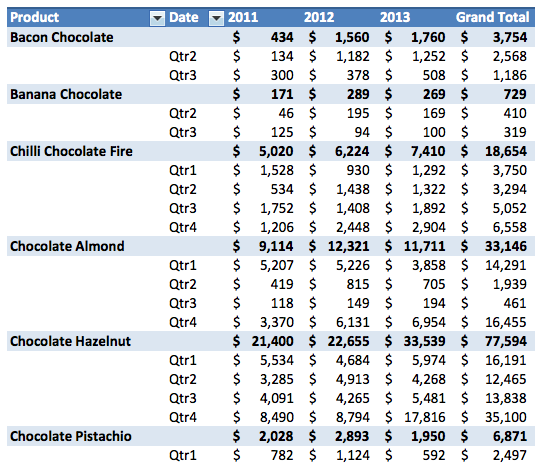
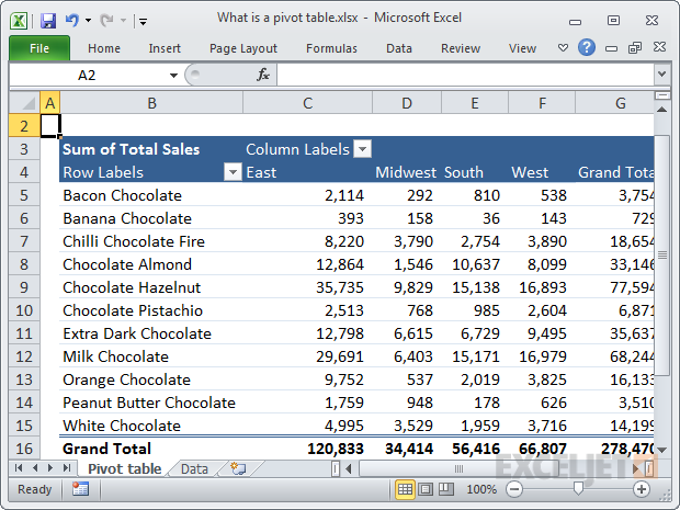
At the most basic level, pivot tables answer important questions. For example, assume you’re working with a company that sells chocolate to retailers and have some sales data that looks something like this:

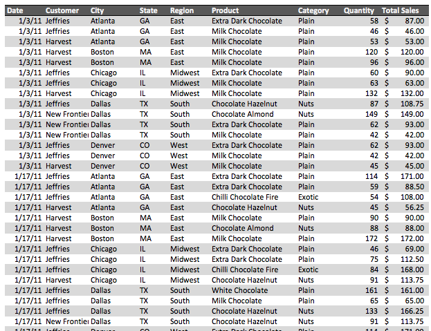
Here are some questions that might be going through your mind:

• What are my best-selling products?
• Who are my biggest customers?
• Where are my sales coming from?
• What are product sales by year?
• What are customer sales by year?

In about 5 minutes, here are the answers a pivot table can give you:

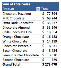
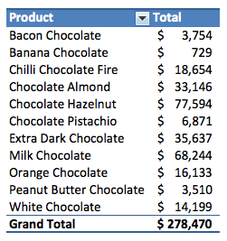
Your top selling products

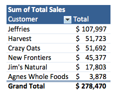
Your biggest customers

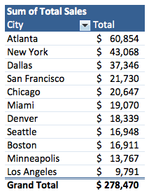
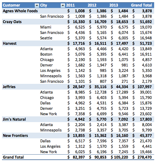
Where sales are coming from

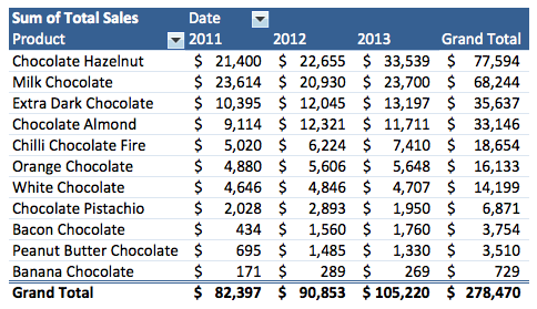
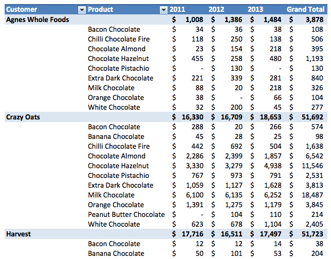
Product sales by year

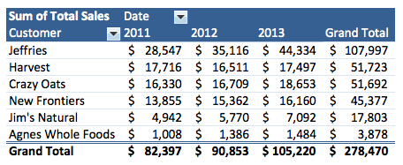
Customer sales by year

Notice that total sales ($278,470) is the same in all pivot tables. Each table presents a different view of the same data, so they all sum to the same number.

So, first and foremost, a pivot table can help you answer questions you have about your data. And in Excel, there is no better tool for this job.

Pivot tables are incredibly fast

Some of you might be thinking: “I could build that summary myself, without pivot tables”. Yes, it’s true. If you have the formula chops to do it, you could create those same reports manually. However, it’s going to take you a lot more time.

In his book, Excel 2013 Pivot Table Data Crunching , Mr. Excel Bill Jelen looks at this very question in detail with one pivot table. With expert skills, he manually builds a basic summary of product sales by region. He concludes:

It took 77 clicks or keystrokes. If you could pull all this off in 5 or 10 minutes, you would probably be fairly proud of your Excel prowess — there were some good tricks among those 77 operations.

Then, he contrasts this with a pivot table approach: a few clicks and done. Watch the video below to see a side-by-side demo of formulas versus pivot tables. No matter how fast you are in Excel, a pivot table will beat you every time.

Video: Formulas vs. Pivot Tables

Pivot tables don’t require formulas

That’s right. Pivot tables don’t require any formulas at all. Not just a few formulas, but zero formulas. Basically, if you can click and drag with a mouse, you can build a pivot table.

To illustrate how truly powerful this is, let’s do something really hard with our pivot table. Let’s group all the orders in the sales data we just looked at into buckets according to the size of the order. That is, we want to see a breakdown of all sales small and large orders.

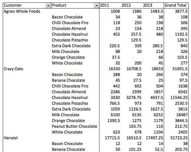
In a couple of minutes, we have a breakdown of orders by order total. This is cool, but useless, because there’s way too much data here:

However, using the built-in group by feature, we can ask Excel to group the orders into buckets of $100. When we click OK, we have a new layout that does this grouping for us perfectly:

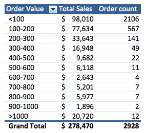
This summary tells us that out of almost 3000 orders, 2106 orders are less than $100, and only 12 orders are greater than $1,000.

Now, consider the formulas it would take to create this kind of report manually. Believe me, they aren’t going to be pretty. Even if you eventually work it out, you won’t understand what they do after a few weeks.

Which brings us to our next point.

Pivot tables don’t make mistakes

Have you ever felt the stress of worrying that your worksheet might contain errors? Maybe you’ve had the unpleasant experience of presenting a report to your management only to have someone find a simple mistake in one of your formulas, casting a shadow on the entire worksheet (and you)?

If so, you’re not alone. These kinds of errors happen all the time, even to pros. Perhaps you read about the spreadsheet mistake that may have impacted the global economy ? It was a basic error. A formula that was supposed to average values for twenty countries only averaged values in 15 countries. So, instead of AVERAGE(L30:L49), the formula said AVERAGE(L30:L44). This is the kind of “silent” problem that can come back to haunt the author of a spreadsheet.

So, how does this relate back to pivot tables? Like this: because pivot tables don’t require you to write formulas, there’s no chance to mess one up. Your only job is to make sure the source data is correct. The pivot table takes care of the rest.

When you work with pivot tables, Excel handles 100% of the calculations and formatting for you. Whether you’re working with 100, 1,000, or 100,000 rows of data, you know the results will be accurate.

Pivot tables make you look good

You’ve probably noticed by now that formatting things in Excel to look good is tricky and time-consuming. And when your boss or client wants to see the report configured differently, you’re back to square one, clearing and re-applying formatting.

Pivot tables are different. All of the formatting they apply is clean and automatic.

For example, let’s look at this plain pivot table with minimal formatting:

A plain pivot table without formatting

With a few clicks, we can transform the entire table into a pro-level report:

The same pivot table after applying a built-in style

Now, if you need to rearrange the table to show cities instead of products, that’s no problem. Excel automatically clears and replies formatting each time it’s changed, without any effort by you:

A new layout, but all formatting is automatically applied

When you use pivot tables, you get a perfectly formatted report every time.

Pivot tables are a great tool for prototyping

Sometimes, you don’t know exactly what you need, given the data you’ve got to work with. A pivot table allows you to experiment fluidly. You can quickly try out different layouts until you find what you need. In fact, for just this reason, pivot tables are an awesome prototyping tool.

For example, maybe you’re supposed to tell IT what kind of report your boss needs for quarterly sales because they need to code it into a web app they manage. Using a pivot table and some sample data, you start off by adding the product and sales to your pivot table:

Next you add in the date, then group by year and quarter:

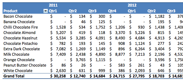
Not bad, but this report is too wide. Maybe quarters would work better in rows?

This will work. Now you have something you can send to the IT guys to show them exactly what they need to build.

Pivot tables are an excellent prototyping tool. They help you understand what data you need to collect and how to present it effectively without long delays and expensive development costs.

Pivot tables can analyze all kinds of data, not just sales data

If you look at the pivot table examples on the web, you’d think that the only thing a pivot table is good for is sales data. Not true. You can use a pivot table to analyze any kind of tabular data.

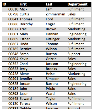
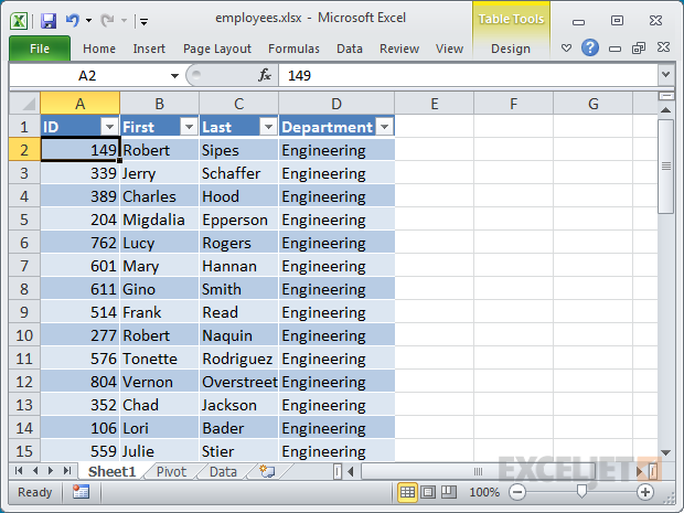
For example, Let’s say you just got an employee list from HR and need to create a simple breakdown by department. Here’s the data:

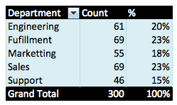
You look at it and realize you can just push it through a pivot table. A minute later, here’s your breakdown by department.

Let’s look at another example. Maybe you work in residential real estate and export a list of 200 properties in a certain location. The data looks like this:

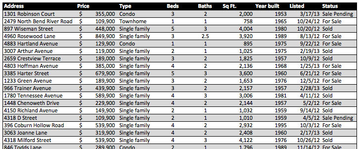
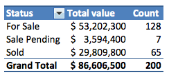
What you want to see is the number of properties that are sold, pending, and for sale. You also want to see the total value of these properties.

30 seconds later, you’ve got your summary:

Do you see the pattern? You start off with raw data, most likely collected by a system of some kind. You pour it into a pivot table, Excel crunches through the data in about, oh, 1 second, and out jumps the essential truths about the data, i.e. the things you need to know.

Pivot tables are easy to update

In the real world, data is always changing.

Unlike most other tools in Excel, pivot tables do not update automatically. This sometimes puzzles new users. They make a change in the source data, check the pivot table, and…nothing. To update a pivot table, you need to refresh the data. Once you start to “get” pivot tables, you’ll realize that refreshing the data is the best part about pivot tables, because it’s the moment when Excel does a lot of work for you.

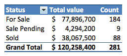
To illustrate, let’s go back to the property-listing example. You have your summary of 200 properties, but you adjust your search a month later, run another data export, and end up with a bigger list that contains 281 properties.

To update your report, here’s what you do. First, you paste over the data you collected previously. Because the data sits in an Excel table, the table range automatically adjusts to include the 81 new properties. Next, you refresh your pivot table, and you’re done. Here’s the result:

Once you’ve set up a pivot table, you can easily update the data at any time. All changes in the data will be reflected in the pivot table, without any work on your part.

Summary

Hopefully, I’ve managed to convince you that pivot tables are a skill you need to know. As the single most powerful feature in Excel, they help you do the following:

1. Answer key questions
2. Work incredibly fast
3. Avoid mistakes
4. Build beautiful reports
5. Quickly prototype reports
6. Handle changes with grace
7. Keep your job

Oh yeah. You probably want to know how the restructuring turned out :)

So, in the end the restructuring was a disaster. Senior management “bet the farm” on a radical idea inspired by the frothy internet start-ups of that era, and they lost, big-time. It took a couple of years, but eventually they ran the company out of money and up on the rocks. During that time, I had to downsize almost every quarter. Finally, a competitor in the UK bought our company at a fire-sale price and initiated their own brutal restructuring (but with a pleasant English accent). By the time that was done, I was the last person from the original office still around.

I won’t say that pivot tables saved my job. It’s not quite that simple. But I do think they played a big role. Because I had key business information for the office in a collection of pivot table reports, I could review these reports with my team, and management at any time. The pivot tables were honestly the only way I was able to understand and communicate what was going on during that crazy period of my career. Without them, I couldn’t have done it.

Want to learn more about pivot tables? We have video training .

Quick Links

• Overview
• Why Pivot?
• Tips
• Examples
• Training

Pivot tables are a reporting engine built into Excel. They are the single best tool in Excel for analyzing data without formulas . You can create a basic pivot table in about one minute, and begin interactively exploring your data. Below are more than 20 tips for getting the most from this flexible and powerful tool.

1. You can build a pivot table in about one minute

Many people think building a pivot table is complicated and time-consuming, but it’s simply not true. Compared to the time it would take you to build an equivalent report manually, pivot tables are incredibly fast. If you have well-structured source data, you can create a pivot table in less than a minute. Start by selecting any cell in the source data:

Example source data

Next, follow these four steps:

1. On the Insert tab of the ribbon, click the PivotTable button
2. In the Create PivotTable dialog box, check the data and click OK
3. Drag a “label” field into the Row Labels area (e.g. customer)
4. Drag a numeric field into the Values area (e.g. sales)

A basic pivot table in about 30 seconds

The pivot table above shows total sales by product, but you can easily rearrange fields to show total sales by region, by category, by month, and so on. Watch the video below for a quick demonstration:

Video: How to quickly create a pivot table

2. Clean your source data

To minimize problems down the road, make sure your data is in good shape. Source data should have no blank rows or columns, and no subtotals. Each column should have a unique name (on one row only) and represent a field for each row/record in the data:

Perfect data for a pivot table!

You might sometimes need to add missing data. See this video for tips:

Video: How to quickly fill in missing data

3. Count the data first

When you first create a pivot table, use it to generate a simple count first to make sure the pivot table is processing the data as you expect. To do this, simply add any text field as a Value field. You’ll see a very small pivot table that displays the total record count, that is, the total number of rows in your data. If this number makes sense to you, you’re good to go. If the number doesn’t make sense to you, it’s possible the pivot table is not reading the data correctly or that the data has not been defined correctly.

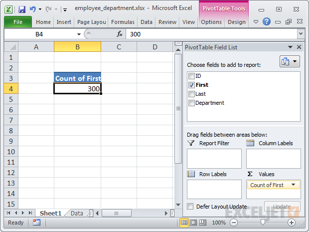
300 first names means we have 300 employees. Check.

4. Plan before you build

Although it’s a lot of fun dragging fields around a pivot table, and watching Excel churn out yet another unusual representation of the data, you can find yourself going down a lot of unproductive rabbit holes very easily. An hour later, it’s not so fun anymore. Before you start building, jot down what you are trying to measure or understand, and sketch out a few simple reports on a notepad. These simple notes will help guide you through the huge number of choices you have at your disposal. Keep things simple, and focus on the questions you need to answer.

5. Use a table for your data to create a “dynamic range”

If you use an Excel Table for the source data of your pivot table, you get a very nice benefit: your data range becomes “dynamic”. A dynamic range will automatically expand and shrink the table as you add or remove data, so won’t have to worry that the pivot table is missing the latest data. When you use a Table for your pivot table, the pivot table will always be in sync with your data.

To use a Table for your pivot table:

1. Select any cell in the data and use the keyboard shortcut Ctrl-T to create a Table
2. Click the Summarize with PivotTable button (TableTools > Design)
3. Build your pivot table normally
4. Profit: data you add to your Table will automatically appear in your Pivot table on refresh

Video: Use a table for your next pivot table

Creating a simple Table from the data using (Ctrl-T)

Now that we have a table, we can use Summarize with a Pivot Table

Still need inspiration on why you should learn pivot tables? See my personal story .

6. Use a pivot table to count things

By default, a Pivot Table will count any text field. This can be a really handy feature in a lot of general business situations. For example, suppose you have a list of employees and want to get a count by department. To get a breakdown by department, follow these steps:

1. Create a pivot table normally
2. Add the Department as a Row Label
3. Add the employee Name field as a Value
4. The pivot table will display a count of employee by Department

Employee breakdown by department

7. Show totals as a percentage

In many pivot tables, you’ll want to show a percentage rather than a count. For example, perhaps you want to show a breakdown of sales by product. But, rather than show the total sales for each product, you want to show sales as a percentage of the total sales. Assuming you have a field called Sales in your data, just follow these steps:

1. Add Product to the pivot table as a Row Label
2. Add Sales to the pivot table as a Value
3. Right-click the Sales field, and set “Show Values As” to “% of Grand Total”

See the tip below “Add a field more than once to a pivot table” to learn how to show total sales and sales as a percent of total at the same time.

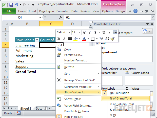
Changing value display to % of total

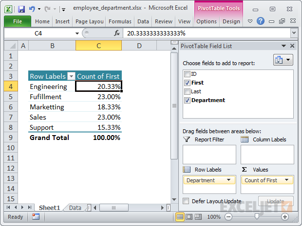
The sum of employees displayed as % of total

8. Use a pivot table to build a list of unique values

Because pivot tables summarize data, they can be used to find unique values in a field. This is a good way to quickly see all the values that appear in a field and also find typos, and other inconsistencies. For example, suppose you have sales data and you want to see a list of every product that was sold. To create a product list:

1. Create a pivot table normally
2. Add the Product as a Row Label
3. Add any other text field (category, customer, etc) as a Value
4. The pivot table will show a list of all products that appear in the sales data

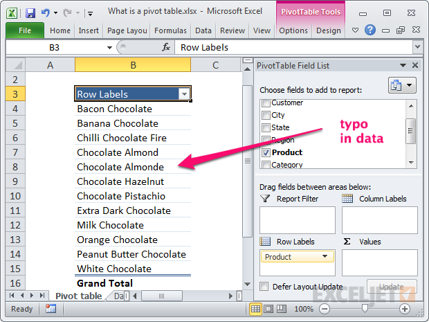
Every product that appears in the data is listed (including a typo)

Pivot Table video training - quick, clean, and to the point

9. Create a self-contained pivot table

When you’ve created a pivot table from data in the same worksheet, you can remove the data if you like and the pivot table will continue to operate normally. This is because a pivot table has a pivot cache that contains an exact duplicate of the data used to create the pivot table.

1. Refresh the pivot table to ensure the cache is up to date (PivotTable Tools > Refresh)
2. Delete the worksheet that contains the data
3. Use your pivot table normally

Video: How to make a self-contained pivot table

10. Group a pivot table manually

Although pivot tables automatically group data in many ways, you can also group items manually into your own custom groups. For example, assume you have a pivot table that shows a breakdown of employees by department. Suppose you want to further group the Engineering, Fulfillment, and Support departments into Group 1, and Sales and Marketing into Group 2. Group 1 and Group 2 don’t appear in the data, they are your own custom groups. To group the pivot table into the ad hoc groups, Group 1 and Group 2:

1. Control-click to select each item in the first group
2. Right-click one of the items and choose Group from the menu
3. Excel creates a new group, “Group1”
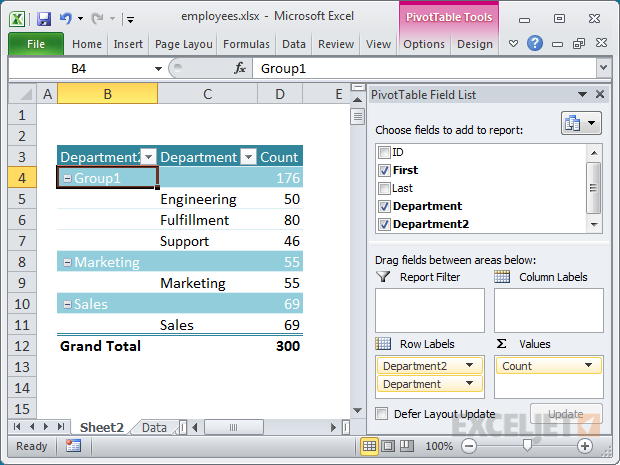
4. Select Marketing and Sales in column B, and group as above
5. Excel creates another group, “Group2”

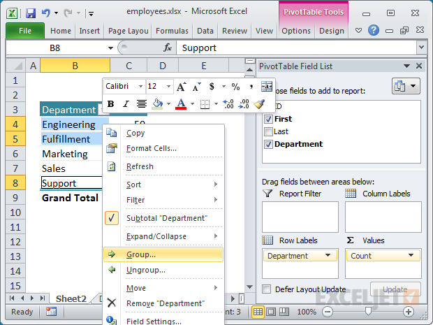
Starting to group manually

Half way through manual grouping - Group 1 is done

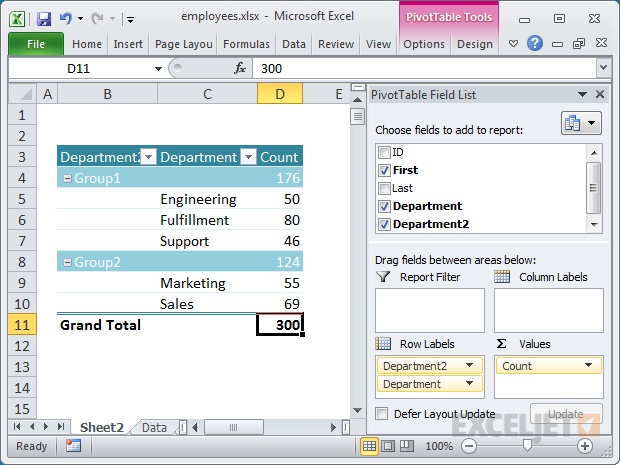
Finished grouping manually

11. Group numeric data into ranges

One of the most interesting and powerful features that every pivot table has is the ability to group numeric data into ranges or buckets. For example, assume you have a list of voting results that includes voter age, and you want to summarize the results by age group:

1. Create your pivot table normally
2. Add Age as a Row Label, Vote as a Column Label, and Name as a Value
3. Right-click any value in the Age field and choose Group
4. Enter 10 as the interval in the “By:” input area
5. When you click OK, you’ll see the voting data grouped by age into 10-year buckets

Video: How to group a pivot table by age range

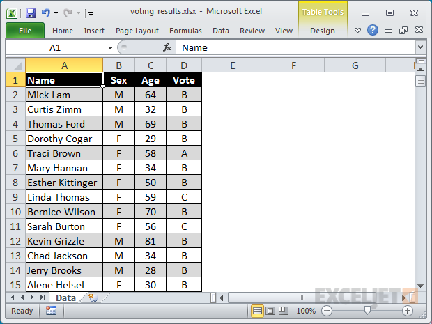
The source data for voting results

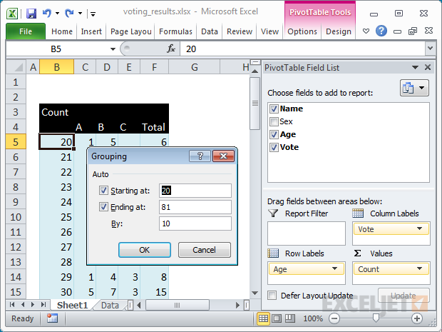
Grouping the age field into 10-year buckets

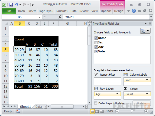
Done grouping voting results by age range

12. Rename fields for better readability

When you add fields to a pivot table, the pivot table will display the name that appears in the source data. Value field names will appear with “Sum of " or “Count of” when they are added to a pivot table. For example, you’ll see Sum of Sales, Count of Region, and so on. However, you can simply overwrite this name with your own. Just select the cell that contains the field you want to rename and type a new name.

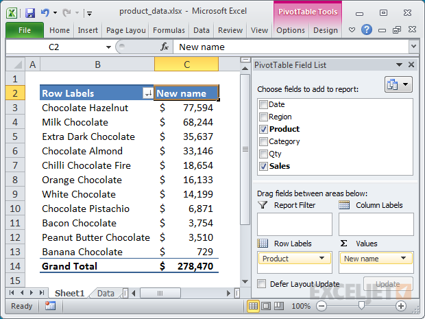
Rename a field by typing over the original name

13. Add a space to field names when Excel complains

When you try to rename fields, you might run into a problem if you try to use exactly the same field name that appears in the data. For example, suppose you have a field called Sales in your source data. As a value field, it appears as Sum of Sales , but (sensibly) you want it to say Sales . However, when you try to use Sales, Excel complains that the field already exists, and throws a “PivotTable field name already exists” error message.

Excel doesn’t like your new field name

As a simple workaround, just add a space to the end of your new field name. You can’t see a difference, and Excel won’t complain.

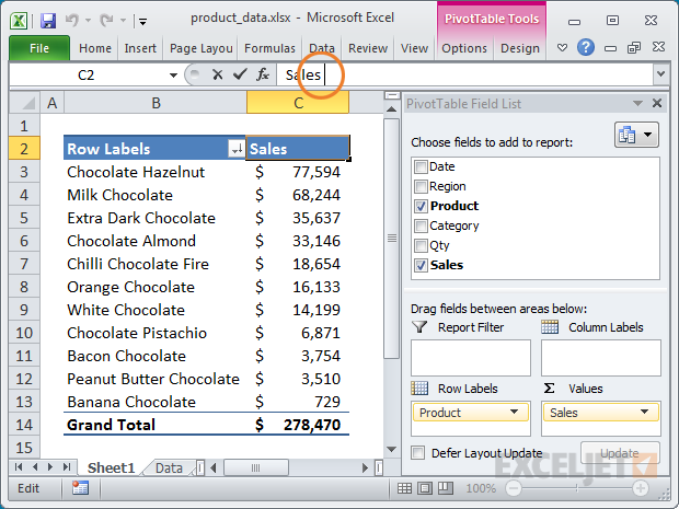
Adding a space to the name avoids the problem

14. Add a field more than once to a pivot table

There are many situations when it makes sense to add the same field to a pivot table more than once. It may seem odd, but you can indeed add the same field to a pivot table more than once. For example, suppose you have a pivot table that shows a count of employees by department.

The count works fine, but you also want to show the count as a percentage of total employees. In this case, the simplest solution is to add the same field twice as a Value field:

1. Add a text field to the Value area (e.g. First name, Name, etc.)
2. By default, you’ll get a count for text fields
3. Add the same field again to the Value area
4. Right-click the second instance, and change Show Values As to “% of Grand Total”
5. Rename both fields as you wish

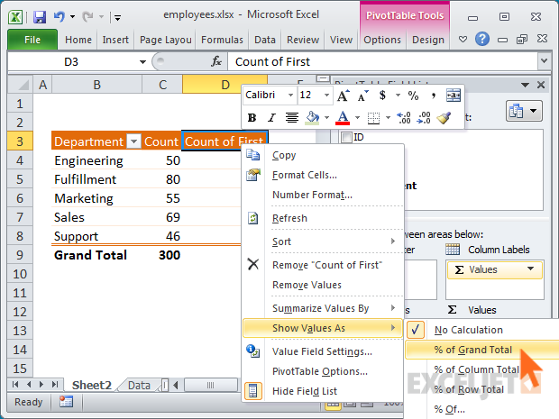
Setting a field to show percent of total

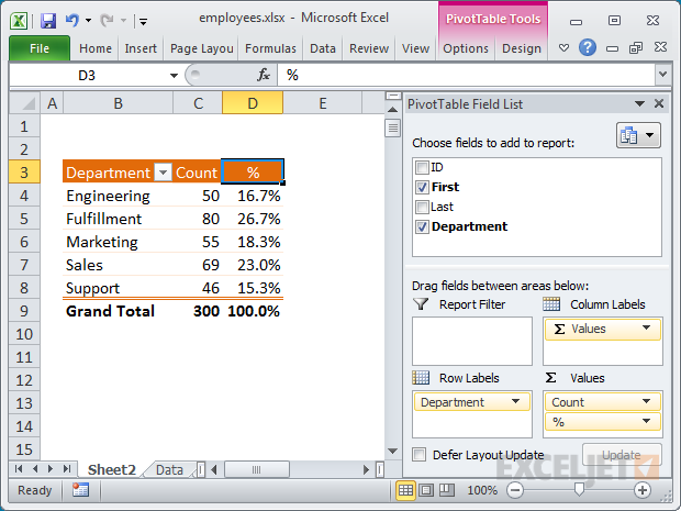
The Name field has been added twice

15. Automatically format all value fields

Any time you add a numeric field as a Value in a pivot table, you should set the number format directly on the field. You may be tempted to format the values you see in the pivot table directly, but this is not a good idea, because it’s not reliable as the pivot table changes. Setting the format directly on the field will ensure that the field is displayed using the format you want, no matter how big or small the pivot table becomes.

For example, assume a pivot table that shows a breakdown of sales by Region. When you first add the Sales field to the pivot table, it will be displayed in General number format, since it’s a numeric field. To apply the Accounting number format to the field itself:

1. Right-click on the Sales field and select Value Field Settings from the menu
2. Click the Number Format button in the Value field settings dialog that appears
3. Set the format to Accounting and click OK to exit

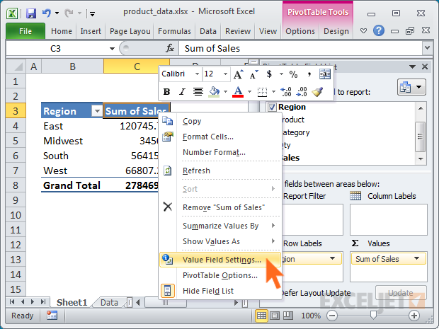
Setting format directly on a value field

16. Drill down to see (or extract) the data behind any total

Whenever you see a total displayed in a pivot table, you can easily see and extract the data that makes up the total by “drilling down”. For example, assume you are looking at a pivot table that shows employee count by department. You can see that there are 50 employees in the Engineering department, but you want to see the actual names. To see the 50 people that make up this number, double-click directly on the number 50, and Excel will add a new sheet to your workbook that contains the exact data used to calculate 50 engineers. You can use this same approach to see and extract data behind totals wherever you see them in a pivot table.

<img loading=“lazy” src=“https://exceljet.net/sites/default/files/styles/original_with_watermark/public/images/articles/inline/drill_down1.png?itok=Yrwa27W7" onerror=“this.onerror=null;this.src=‘https://blogger.googleusercontent.com/img/a/AVvXsEhe7F7TRXHtjiKvHb5vS7DmnxvpHiDyoYyYvm1nHB3Qp2_w3BnM6A2eq4v7FYxCC9bfZt3a9vIMtAYEKUiaDQbHMg-ViyGmRIj39MLp0bGFfgfYw1Dc9q_H-T0wiTm3l0Uq42dETrN9eC8aGJ9_IORZsxST1AcLR7np1koOfcc7tnHa4S8Mwz_xD9d0=s16000';" alt=“Double click a total to “drill down” - 43”>

Double click a total to “drill down”

The 50 Engineers, extracted into a new sheet automatically

17. Clone your pivot tables when you need another view

Once you have one pivot table set up, you might want to see a different view of the same data. You could of course just rearrange your existing pivot table to create the new view. But if you’re building a report that you plan to use and update on an ongoing basis, the easiest thing to do is clone an existing pivot table, so that both views of the data are always available.

There are two easy ways to clone a pivot table. The first way involved duplicating the worksheet that holds the pivot table. If you have a pivot table set up in a worksheet with a title, etc., you can just right-click the worksheet tab to copy the worksheet into the same workbook. Another way to clone a pivot table is to copy the pivot table and paste it somewhere else. Using these approaches, you can make as many copies as you like.

When you clone a pivot table this way, both pivot tables share the same pivot cache . This means that when you refresh any one of the clones (or the original) all of the related pivot tables will be refreshed.

Video: How to clone a pivot table

18. Un-clone a pivot table to refresh independently

After you’ve cloned a pivot table, you might run into a situation where you really don’t want the clone to be linked to the same pivot cache as the original. A common example is after you’ve grouped a date field in one pivot table, refresh, and discover that you’ve also accidentally grouped the same date field in another pivot table that you didn’t intend to change. When pivot tables share the same pivot cache, they also share field grouping as well.

Here’s one way to un-clone a pivot table, that is, unlink it from the pivot cache it shares with other pivot tables in the same worksheet:

1. Cut the entire pivot table to the clipboard
2. Paste the pivot table into a brand-new workbook
3. Refresh the pivot table
4. Copy it again to the clipboard
5. Paste it back into the original workbook
6. Discard the temporary workbook

Your pivot table will now use its own pivot cache and will not refresh with the other pivot table(s) in the workbook, or share the same field grouping.

19. Get rid of useless headings

The default layout for new pivot tables is the Compact layout. This layout will display “Row Labels” and “Column Labels” as headings in the pivot table. These aren’t the most intuitive headings, especially for people who don’t often use pivot tables. An easy way to get rid of these odd headings is to switch the pivot table layout from Compact to Outline or Tabular layout. This will cause the pivot table to display the actual field names as headings in the pivot table, which is much more sensible. To get rid of these labels altogether, look for a button called Field Headers on the Analyze tab of the Pivot Table Tools ribbon. Clicking this button will disable headings completely.

Note the useless and confusing field headings

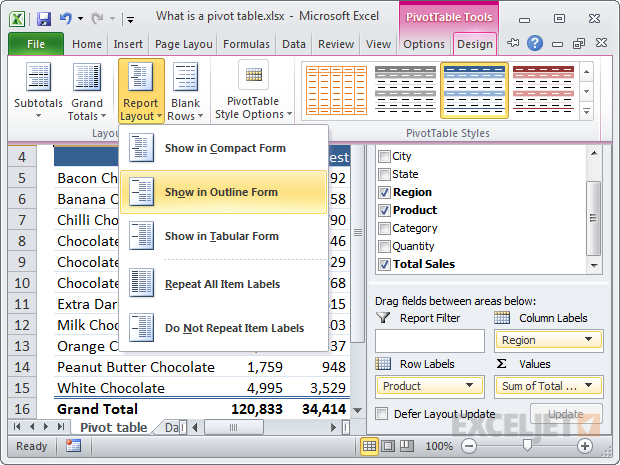
Switching the layout from Compact to Outline

Field headings in the Outline layout are much more sensible

20. Add a little white space around your pivot tables

This is just a simple design tip. All good designers know that a pleasing design requires a little white space. White space just means empty space set aside to give the layout breathing room. After you create a pivot table, insert an extra column to the left and an extra row or two at the top. This will give your pivot table some breathing room and create a better looking layout. In most cases, I also recommend that you turn off gridlines on the worksheet. The pivot table itself will present a strong visual grid, so the gridlines outside the pivot table are unnecessary, and will simply create visual noise.

A little white space makes your pivot tables look more polished

Inspiration: 5 pivot tables you haven’t seen before .

21. Get rid of row and column grand totals

By default, pivot tables show totals for both rows and columns, but you can easily disable one or both of these totals if you don’t want them. On the Pivot Table tab of the ribbon, just click the Totals button and choose the options you want.

You can remove grand totals for both rows and columns

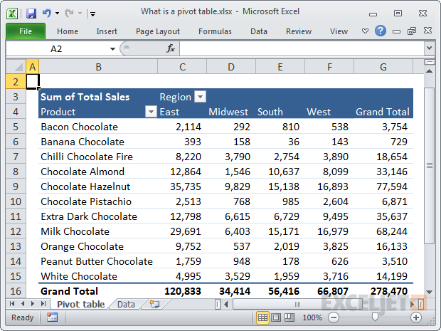
22. Format empty cells

If you have a pivot table that has a lot of blank cells, you can control the character that is displayed in each blank cell. By default, empty cells will display nothing at all. To set your own character, right-click inside the pivot table and select Pivot Table options. Then make sure that “Empty cells as:” is checked, and enter the character you want to see. Keep in mind that this setting respects the applied number format. For example. if you are using the accounting number format for a numeric value field, and enter a zero, you’ll see a hyphen “-” displayed in the pivot table, since that’s how zero values are displayed with the Accounting format.

Empty cells set to display 0 (zero) and Accounting number format gives you hyphens

23. Turn off AutoFit when necessary

By default, when you refresh a pivot table, the columns that contain data are adjusted automatically to best fit the data. Normally, this is a good thing, but it can drive you crazy if you have other things on the worksheet along with the pivot table, or if you have carefully adjusted the column widths manually and don’t want them changed. To disable this feature, right-click inside the pivot table and choose PivotTable Options. In the first tab of the options (or the layout tab on a Mac), uncheck “AutoFit Column Widths on Update”.

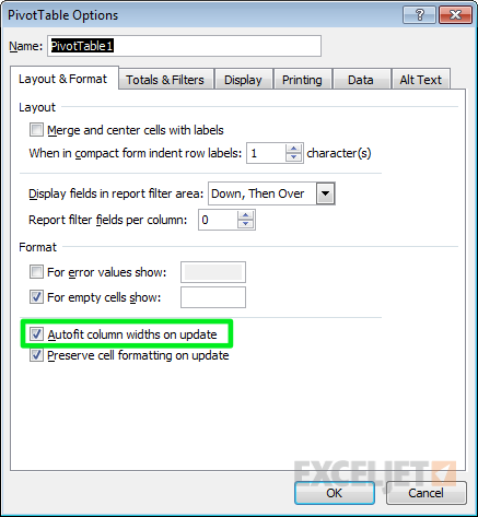
Pivot table column autofit option for Windows

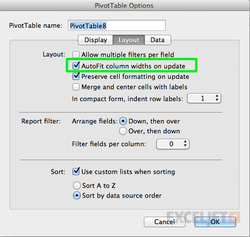
Pivot table column autofit option for Mac

Need to learn Pivot Tables? We have solid video training with practice worksheets.