Explanation
In this example, the goal is to return a TRUE or FALSE result for each value in column B, based on whether it appears in the range E5:E9, which has been named “things” for convenience.
Context
Imagine you have a list of values in the range B5:B16 and you want to check each value to see if it appears in another list of values in the range E5:E9, which has been named “things”. You might think you can use a formula like this:
=B5=things
However, because we are comparing B5 to the range E5:E9, which contains five values, the formula will return five results. With “green” in cell B5, the result will be an array like this:
{FALSE;FALSE;TRUE;FALSE;FALSE}
And if we copy the formula down, each value in column B will return five results. This idea isn’t going to work as-is. You could build a more complicated formula using nested IF statements to check for each value separately, but this is a tricky path that will take much longer and greatly increase the chance of errors. A much simpler, cleaner approach is to use an array formula based on the SUMPRODUCT function.
Solution with SUMPRODUCT
The SUMPRODUCT function multiplies ranges or arrays together and returns the sum of products. This sounds boring, but SUMPRODUCT is a versatile function that can be used to solve many tricky problems in Excel. It works nicely in this case because it can handle arrays natively in any version of Excel.
Note: In Excel 2021 or Excel 365, you can use the SUM function instead of SUMPRODUCT and it will just work fine. However, if the worksheet is opened in an older version of Excel, it will appear as a traditional array formula surrounded by curly braces. If you need backward compatibility, SUMPRODUCT avoids this complication and works the same in all versions.
Back to the problem. As mentioned above, if we compare the value in cell B5 directly with the values in things (E5:E9), we get back an array that contains five TRUE or FALSE values. This seems inconvenient because it isn’t obvious how we can resolve this list of five results into a single TRUE or FALSE value. However, we can use SUMPRODUCT to process the array of TRUE/FALSE values and return a single result with a formula like this:
=SUMPRODUCT(--(B5=things))>0
At a high level, this formula counts the TRUE values in the array and then checks if the result is greater than zero. Working from the inside out, the expression B5=things returns five values, as explained above.
=B5=things // returns {FALSE;FALSE;TRUE;FALSE;FALSE}
If we simplify the formula, we now have:
=SUMPRODUCT(--({FALSE;FALSE;TRUE;FALSE;FALSE}))>0
You might wonder what the double negative (–) is doing here. SUMPRODUCT is designed to process numeric values, and it will simply ignore TRUE and FALSE values. If we try to use the raw values, SUMPRODUCT will return zero:
=SUMPRODUCT(FALSE;FALSE;TRUE;FALSE;FALSE}) // returns 0
The double negative (–) is a simple trick to force Excel to convert the TRUE and FALSE values to their numeric equivalents, 1 and 0. After this operation is evaluated, we can simplify the formula to this:
=SUMPRODUCT({0;0;1;0;0})>0
Notice that each FALSE value in the array is now zero, and the lone TRUE in the array is now 1. Now you can see where we are headed. Since the array contains only numbers, SUMPRODUCT will return a sum. If we get any non-zero result, we have a match, so we use >0 to force a final result of either TRUE or FALSE:
=SUMPRODUCT({0;0;1;0;0})>0
=1>0
=TRUE
With a hard-coded list
There’s no requirement to use a range for your list of things to check for. If you’re only looking for a small number of things, you can use a list in array format, which is called an array constant . For example, if you’re just looking for the colors red, blue, and green, you can use {“red”,“blue”,“green”} like this:
=SUMPRODUCT(--(B5={"red","blue","green"}))>0
Using a range is a more flexible approach since the values appear on the worksheet and can be changed at any time.
Dealing with extra spaces
If the cells you are testing contain any extra space, they won’t match properly. To strip all extra space, you can modify the formula to use the TRIM function like so:
=SUMPRODUCT(--(TRIM(A1)=things))>0
TRIM will strip leading or trailing space characters from the value before it is compared to the list of things.
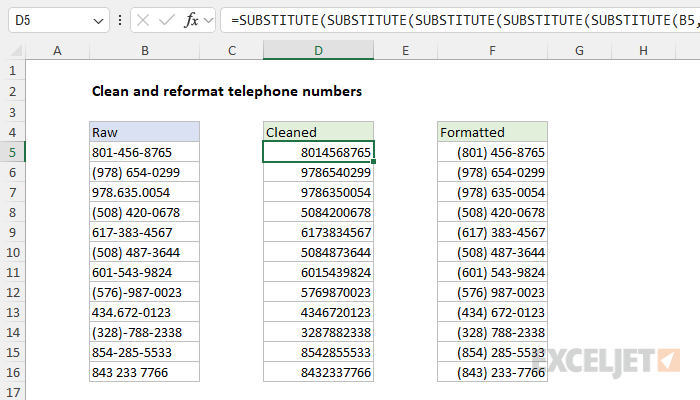
Explanation
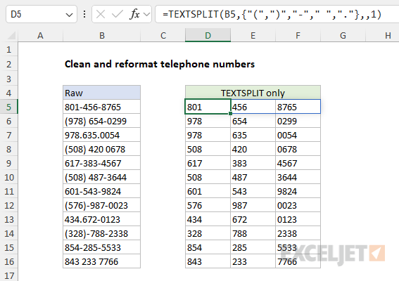
In this example, the goal is to clean up telephone numbers with inconsistent formatting and then reformat the numbers in the same way. In practice, this means we need to start by removing the extra non-numeric characters, including spaces, dashes, periods, and parentheses. Once these characters are removed, we can use Excel’s number format system to format the numbers consistently. In the worksheet shown, the formula used to learn the numbers looks like this:
=TEXTJOIN("",1,TEXTSPLIT(B5,{"(",")","-"," ","."},,1))+0
- Removing extra characters
- Joining the numbers with punctuation
- Creating a single numeric value
- Applying number formatting with Format Cells
- Applying number formatting with the TEXT function
- All in one spill formula with the BYROW function
- Formula for older versions of Excel
- Line wrap trick for better readability
Removing extra characters
The first task is to remove the extra characters in the raw telephone numbers. These include the right and left parentheses “()”, dashes or hyphens “-”, space characters " “, and periods “.”. The traditional approach to removing more than one value in an Excel formula is to nest together multiple SUBSTITUTE functions (see details below). However, since we have a limited number of characters to remove, a clever approach in this case is to use the TEXTSPLIT function like this:
TEXTSPLIT(B5,{"(",")","-"," ","."},,1)
Where the inputs to TEXTSPLIT are as follows:
- text - the text in cell B5
- col_delimiter - the array constant {”(",")","-"," “,”."}
- row_delimiter - omitted
- ignore_empty - 1 (same as TRUE)
The key in this formula is the array constant with five values. Essentially, we are asking TEXTSPLIT to split the text at each parenthesis, dash, space, and period. We are also asking TEXTSPLIT to ignore any empty values that are generated. This is important because some of these delimiters have no actual value between them. The result is that the original telephone numbers are neatly split into three parts, and all five delimiters have been removed:
What’s interesting about this (to me at least) is that when you use TEXTSPLIT to split text with different delimiters, the delimiters themselves are discarded in the process . This makes TEXTSPLIT an interesting way to remove multiple characters at the same time. The only drawback is that you have to combine the split text again, which is why we have TEXTJOIN in there as well. The CONCAT function would work equally well to join the numbers.
Note: if you have a lot of characters to remove, you can use a different formula to strip all non-numeric values at once , without calling out individual characters.
Joining the numbers with punctuation
To create a final formatted result, one approach is to use manual concatenation to join the numbers together using the exact syntax you prefer. For example, in the screen below, the formula in cell H5 is:
="("&D5&") "&E5&" -"&F5
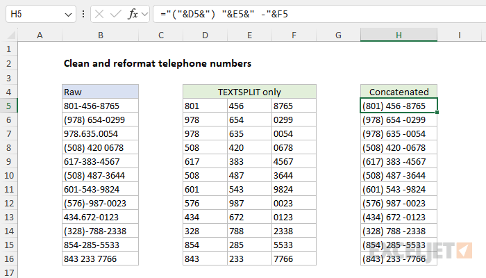
The key benefit of this approach is total control over the final result. You can insert specific characters with any logic you like. However, in the original worksheet shown above, we take a different approach: we create a single number, and then apply number formatting.
Creating a single numeric value
After the TEXTSPLIT splits the numbers and removes delimiters, the resulting array is returned to the TEXTJOIN function like this:
=TEXTJOIN("",1,{"801","456","8765"})+0
Because we have provided an empty string as the delimiter, the result from TEXTJOIN is a single text string like this:
="8014568765"+0
We then add zero to force Excel to convert the text value to the number 8014568765. Note: leading zeros will be removed when the value is converted to a number. If you need leading zeros, the simplest approach will be to concatenate manually as explained previously. There are pros and cons to both approaches.
Applying number formatting with Format Cells
The final step in this problem is to apply Excel’s built-in telephone number format. To show this as a separate step, the worksheet below just pulls the value from column D into column F:
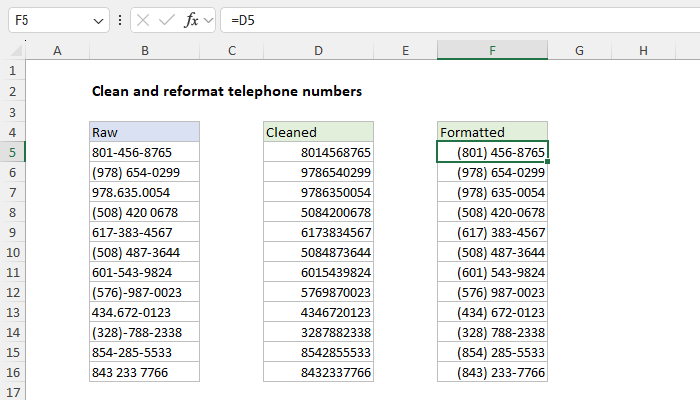
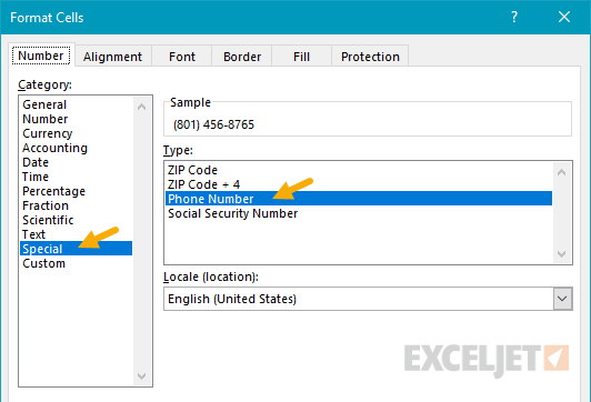
Next, select the range F5:F16 and use the keyboard shortcut Control + 1 to open the Format Cells window. Then apply the “Phone Number” format:
Applying number formatting with the TEXT function
Another good way to apply number formatting is to use the TEXT function with a custom number format like this:
TEXT(A1,"(000) 000-0000")
The result from TEXT will be a text string with the number in a format like (877) 437-8365.
All-in-one spill formula with the BYROW function
=LET(
phoneList,B5:B16,
cleanList,BYROW(phoneList,LAMBDA(n,LET(chars,MID(n,SEQUENCE(LEN(n)),1),CONCAT(FILTER(chars,ISNUMBER(chars+0)))))),
validLen,IFERROR(LEN(cleanList),0)=10,
return,IF(validLen,TEXT(cleanList,"(000) 000-0000"),"Missing or invalid number."),
return
)
Unlike the original formula, which removes specific punctuation, this formula uses the FILTER function with the CONCAT function to strip all non-numeric characters . This code is packaged in a custom LAMBDA function called by the BYROW function , which iterates through all phone numbers one row at a time. It also features a nice error-checking step to confirm a 10-digit number and bail out with a friendly message when a number is not 10 digits. Note the definition of the “validLen” variable in the code above and how it is used in the next line.
Formula for older versions of Excel
Older versions of Excel do not provide the TEXTJOIN or TEXTSPLIT function, so we need a different formula. One traditional approach is to nest multiple SUBSTITUTE functions in a single formula like this:
=SUBSTITUTE(SUBSTITUTE(SUBSTITUTE(SUBSTITUTE(SUBSTITUTE(B5,"(",""),")",""),"-","")," ",""),".","")+0
The formula runs from the inside out, with each SUBSTITUTE removing one character. The innermost SUBSTITUTE removes the left parentheses, and the result is handed to the next SUBSTITUTE, which removes the right parentheses, and so on. The workbook below shows the formula in action:
Whenever you use the SUBSTITUTE function, the result will be text. Because you can’t apply a number format to text, we need to convert the text to a number. One way to do that is to add zero (+0), which automatically converts numbers in text format to numbers in numeric format. Finally, the “Special” telephone number format is applied to column D as explained above.
This page explains custom number formats with many examples.
Line wrap trick for better readability
When nesting multiple functions, it can be difficult to read the formula and keep all parentheses balanced. Excel doesn’t care about extra white space in a formula, so you can add line breaks in the formula to make the formula more readable. For example, the formula above can be written as follows:
=
SUBSTITUTE(
SUBSTITUTE(
SUBSTITUTE(
SUBSTITUTE(
SUBSTITUTE(
A1,
"(",""),
")",""),
"-",""),
" ",""),
".","")
Note that the cell appears in the middle, with function names above and substitutions below. Not only does this make the formula easier to read, but it also makes it easier to add and remove substitutions. You can use this same trick to make nested IF statements easier to read as well.
