Purpose
Return value
Syntax
=CHOOSECOLS(array,col_num1,[col_num2],...)
- array - The array to extract columns from.
- col_num1 - The numeric index of the first column to return.
- col_num2 - [optional] The numeric index of the second column to return.
Using the CHOOSECOLS function
The Excel CHOOSECOLS function returns specific columns from an array or range . The columns to return are provided as numbers in separate arguments. Each number corresponds to the numeric index of a column in the source array. The result from CHOOSECOLS is always a single array that spills onto the worksheet.
The first argument in the CHOOSECOLS function is the array , which can be a range, an array constant, or an array generated by another formula. Additional arguments are in the form: col_num1 , col_num2 , col_num3 , etc., and should be the numeric index of the column to extract.
Basic usage
To get columns 1 and 3 from an array, you can use CHOOSECOLS like this:
=CHOOSECOLS(A1:C5,1,3) // columns 1 and 3
To get the same two columns in reverse order:
=CHOOSECOLS(A1:C5,3,1) // columns 3 and 1
CHOOSECOLS will return a #VALUE! error if a requested column number is out of range:
=CHOOSECOLS(A1:C5,4) // returns #VALUE!
With an array constant
Another option for specifying which columns to return is to use an array constant like {1,2,3} as the second argument ( col_num1) . In the example below, the formula in H3 is:
=CHOOSECOLS(B3:F9,{1,3,5})
With the array constant {1,3,5} given as the second argument, CHOOSECOLS returns columns 1, 3, and 5:

The array constant provided can be in the form {1,2,3} or {1;2;3}.
With negative column numbers
A nice feature of CHOOSECOLS is that you can use negative column numbers to extract columns from the end of a range. For example, to get the last column of a range, you can use a formula like this:
=CHOOSECOLS(range,-1)
To get the second-to-last column, you can use:
=CHOOSECOLS(range,-2)
To get the last three columns in the order that they appear:
=CHOOSECOLS(range,-3,-2,-1)
You can also mix negative and positive row numbers. To return the first and last columns at the same time:
=CHOOSECOLS(range,1,-1)
With arrays
As seen above, you can use an array constant as the second argument in CHOOSECOLS to specify columns. You can also use an array generated with a formula. For example, in the worksheet below, we use the SEQUENCE function inside CHOOSECOLS to reverse the column order of the range B3:D9 with a formula like this in cell F3:
=CHOOSECOLS(B3:D9,-SEQUENCE(COLUMNS(B3:D9)))
Since the range B3:D9 contains 3 columns, COLUMNS returns 3 and SEQUENCE returns {1;2;3}:
SEQUENCE(3) // returns {1;2;3}
The negative sign before SEQUENCE converts the array to {-1;-2;-3}:
-SEQUENCE(3) // returns {-1;-2;-3}
Simplifying, the final CHOOSECOLS formula looks like this:
=CHOOSECOLS(B3:D9,{-1;-2;-3})
The result is that CHOOSECOLS returns the 3 columns in B3:D9 in reverse order:
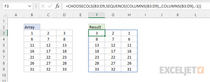
The CHOOSECOLS returns all columns in the array: the last column (-1), the second to last column (-2), and the third to last column (-3).
Notes
- CHOOSECOLS will return a #VALUE error if a column number is out of range.
Purpose
Return value
Syntax
=CHOOSEROWS(array,row_num1,[row_num2],...)
- array - The array to extract rows from.
- row_num1 - The numeric index of the first row to return.
- row_num2 - [optional] The numeric index of the second row to return.
Using the CHOOSEROWS function
The Excel CHOOSEROWS function returns specific rows from an array or range . The rows to return are provided as numbers in separate arguments. Each number corresponds to the numeric index of a row in the source array. The result from CHOOSEROWS is always a single array that spills onto the worksheet.
The first argument in the CHOOSEROWS function is array . Array can be a range, or an array from another formula. Additional arguments are in the form row _num1 , row _num2 , row _num3 , etc. Each number represents a specific row to extract from the array, and should be supplied as a whole number.
Basic usage
To get rows 1 and 3 from an array, you can use CHOOSEROWS like this:
=CHOOSEROWS(A1:A5,1,3) // rows 1 and 3
To get the same two rows in reverse order:
=CHOOSEROWS(A1:A5,3,1) // rows 3 and 1
CHOOSEROWS will return a #VALUE! error if a requested row number is out of range:
=CHOOSEROWS(A1:A5,6) // returns #VALUE!
With array constants
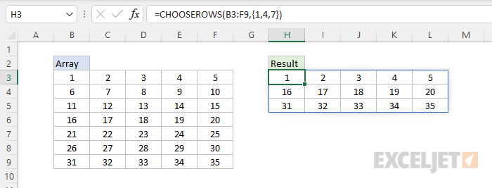
Another option for specifying which rows to return is to use an array constant like {1,4,7} as the second argument ( row_num1) . In the example below, the formula in H3 is:
=CHOOSEROWS(B3:F9,{1,4,7})
With the array constant {1,4,7} given as the second argument, CHOOSEROWS returns rows 1, 4, and 7:
The array constant can be provided in the form {1,2,3} or {1;2;3}.
With negative row numbers
A nice feature of CHOOSEROWS is that you can use negative row numbers to extract rows from the end of a range. For example, to get the last row of a range, you can use a formula like this:
=CHOOSEROWS(range,-1)
To get the second to last row, you can use:
=CHOOSEROWS(range,-2)
To get the last three rows in the order that they appear:
=CHOOSEROWS(range,-3,-2,-1)
You can also mix negative and positive row numbers. To return the first and last row at the same time:
=CHOOSEROWS(range,1,-1)
With arrays
As seen above, you can use an array constant as the second argument in CHOOSEROWS to indicate rows. You can also use an array created with a formula. For example, the formula below uses CHOOSEROWS and the SEQUENCE function to reverse the order of rows in an array:
=CHOOSEROWS(B3:D9,SEQUENCE(ROWS(B3:D9),,ROWS(B3:D9),-1))
When given a 7-row range or array, SEQUENCE returns {7;6;5;4;3;2;1} to CHOOSEROWS, and CHOOSEROWS returns the 7 rows in reverse order:
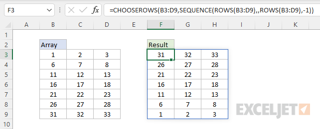
The formula returns all the rows in Array, starting with the last row.
Notes
- CHOOSEROWS will return a #VALUE error if a row number is out of range.
