Purpose
Return value
Syntax
=CHOOSEROWS(array,row_num1,[row_num2],...)
- array - The array to extract rows from.
- row_num1 - The numeric index of the first row to return.
- row_num2 - [optional] The numeric index of the second row to return.
Using the CHOOSEROWS function
The Excel CHOOSEROWS function returns specific rows from an array or range . The rows to return are provided as numbers in separate arguments. Each number corresponds to the numeric index of a row in the source array. The result from CHOOSEROWS is always a single array that spills onto the worksheet.
The first argument in the CHOOSEROWS function is array . Array can be a range, or an array from another formula. Additional arguments are in the form row _num1 , row _num2 , row _num3 , etc. Each number represents a specific row to extract from the array, and should be supplied as a whole number.
Basic usage
To get rows 1 and 3 from an array, you can use CHOOSEROWS like this:
=CHOOSEROWS(A1:A5,1,3) // rows 1 and 3
To get the same two rows in reverse order:
=CHOOSEROWS(A1:A5,3,1) // rows 3 and 1
CHOOSEROWS will return a #VALUE! error if a requested row number is out of range:
=CHOOSEROWS(A1:A5,6) // returns #VALUE!
With array constants
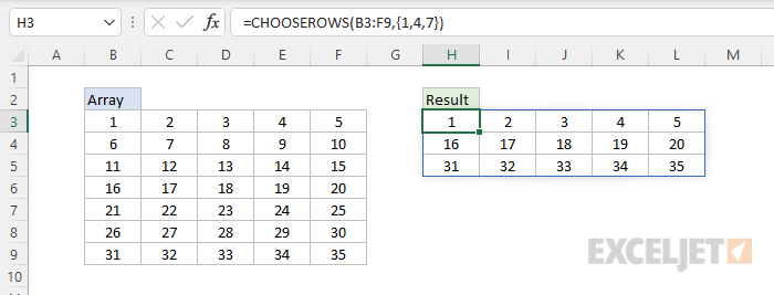
Another option for specifying which rows to return is to use an array constant like {1,4,7} as the second argument ( row_num1) . In the example below, the formula in H3 is:
=CHOOSEROWS(B3:F9,{1,4,7})
With the array constant {1,4,7} given as the second argument, CHOOSEROWS returns rows 1, 4, and 7:
The array constant can be provided in the form {1,2,3} or {1;2;3}.
With negative row numbers
A nice feature of CHOOSEROWS is that you can use negative row numbers to extract rows from the end of a range. For example, to get the last row of a range, you can use a formula like this:
=CHOOSEROWS(range,-1)
To get the second to last row, you can use:
=CHOOSEROWS(range,-2)
To get the last three rows in the order that they appear:
=CHOOSEROWS(range,-3,-2,-1)
You can also mix negative and positive row numbers. To return the first and last row at the same time:
=CHOOSEROWS(range,1,-1)
With arrays
As seen above, you can use an array constant as the second argument in CHOOSEROWS to indicate rows. You can also use an array created with a formula. For example, the formula below uses CHOOSEROWS and the SEQUENCE function to reverse the order of rows in an array:
=CHOOSEROWS(B3:D9,SEQUENCE(ROWS(B3:D9),,ROWS(B3:D9),-1))
When given a 7-row range or array, SEQUENCE returns {7;6;5;4;3;2;1} to CHOOSEROWS, and CHOOSEROWS returns the 7 rows in reverse order:
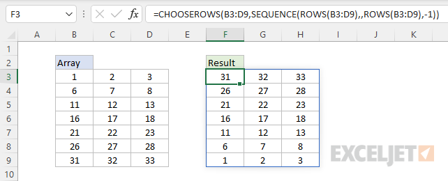
The formula returns all the rows in Array, starting with the last row.
Notes
- CHOOSEROWS will return a #VALUE error if a row number is out of range.
Purpose
Return value
Syntax
=DETECTLANGUAGE(text)
- text - A sample of the language as a text string.
Using the DETECTLANGUAGE function
The DETECTLANGUAGE figures the language for a given text string. The result from DETECTLANGUAGE is a short language code indicating the language. For example, if the language is English, the result is “en”; if the language is French, the result is “fr”; if the language is Japanese, the result is “ja”, and so on. Some of these codes are intuitive, but some aren’t. See below for a list of common language codes. DETECTLANGUAGE only accepts one argument, text, so the syntax is very simple and looks like this:
=DETECTLANGUAGE(text)
Typically, the text is supplied as a cell reference like A1, but it can also be hardcoded as a string like “apple”.
The DETECTLANGUAGE function uses Microsoft Translation Services, so it requires an internet connection.
Basic Example
To use the DETECTLANGUAGE function, simply provide some text. For example, if we give DETECTLANGUAGE the word “apple”, it “detects” English and returns “en”:
=DETECTLANGUAGE("apple") // returns "en"
Likewise, if we give DETECTLANGUAGE the word for “apple” in four languages (French, Italian, German, and Spanish), it returns the four corresponding language codes: “fr,” “it,” “de,” and “es.”
=DETECTLANGUAGE("pomme")  //  returns "fr"
=DETECTLANGUAGE("mela")  //  returns "it"
=DETECTLANGUAGE("Apfel")  //  returns "de"
=DETECTLANGUAGE("manzana")  //  returns "es"
Note that DETECTLANGUAGE always returns a language code like “en”, “it”, “de”, “es”, etc. The TRANSLATE function supports over 100 languages, so there are many potential codes. See below for a list of common languages and codes.
Example: Get language codes
In the worksheet below, we have text for “Is there a coffee shop around here?” in 12 languages. The goal is to determine the language codes based on the text in column B. The formula in D8, copied down, looks like this:
=DETECTLANGUAGE(B5)
As the formula is copied down the column, DETECTLANGUAGE returns a language code for each text string, as seen in column D below:

Note that the DETECTLANGUAGE function is dynamic. If any of the text in column B is changed to a different language, TRANSLATE will return a new language code.
Example: Get language names
Getting language codes automatically is great, but you probably want to know how to get an actual language name. To do that, you will want to set up a lookup table in your worksheet with columns for the language code and the language name. In the worksheet below, we have defined an Excel Table called “languages” like this:

Then we can use the XLOOKUP function to get the correct language for a given code, as seen in column E of the worksheet below. The formula in cell E5 looks like this:
=XLOOKUP(D5,languages[Code],languages[Language])
The inputs to XLOOKUP are as follows:
- lookup_value - D5
- lookup_array - languages[Code]
- return_array - languages[Language]

If you want to look up the language name from the code in one step, you can combine the formulas above into one formula like this:
=XLOOKUP(DETECTLANGUAGE(B5),languages[Code],languages[Language])
In this formula, DETECTLANGUAGE returns a language code to XLOOKUP as the lookup value, and XLOOKUP uses the code to get the language name in a single step.
Excel Tables make it possible to use “structured references” in formulas, like languages[Code] and languages[Language]. One advantage to structured references is that we don’t need to lock any references in a formula like this. To learn more see our Excel Table guide .
Codes for common languages
The below shows language codes for some common languages that can be used with the TRANSLATE function. Note that some languages, like Portuguese, have more than one variant. For example, the code “pt” specifies Portuguese for Brazil, while “pt-pt” specifies Portuguese for Portugal.
| Language | Code | Notes |
|---|---|---|
| Arabic | ar | |
| Chinese | zh-Hans | Simplified |
| Czech | cs | |
| Danish | da | |
| Dutch | nl | |
| English | en | |
| Finnish | fi | |
| French | fr | |
| German | de | |
| Hindi | hi | |
| Indonesian | id | |
| Italian | it | |
| Japanese | ja | |
| Korean | ko | |
| Norwegian | nb | Bokmål |
| Polish | pl | |
| Portuguese | pt | Brazilian |
| Spanish | es | |
| Swedish | sv | |
| Thai | th | |
| Vietnamese | vi |
The DETECTLANGUAGE function supports over 130 languages. You can find the full list of supported languages here .
Notes
- DETECTLANGUAGE always returns a language code as text.
- If the text is an empty string (""), DETECTLANGUAGE also returns an empty string.
- If the internet is not available, you may see a #CONNECT! error.
- Use the TRANSLATE function to translate text to another language.
