Explanation
In this example, the goal is to combine ranges. With the introduction of the VSTACK function and the HSTACK function, this is quite a simple task. To combine ranges vertically, stacking one range on top of another, you can use the VSTACK function like this:
=VSTACK(range1,range2)
To combine ranges horizontally, you can use the HSTACK function like this:
=HSTACK(range1,range2)
In both formulas above, range1 (B5:B8) and range2 (D5:D9) are named ranges . The named ranges are for convenience only, you can use the raw cell references with the same result. For details on how these functions work see our documentation here: VSTACK function , HSTACK function .
Manual approach
Before the VSTACK and HSTACK functions where introduced, but after dynamic array formulas were available , it was possible to combine ranges with a more complex formula using the SEQUENCE function together with the LET function, the INDEX function, and the IF function. This is a much more manual approach, but it is an interesting example of how you can iterate through cells in a range keeping track of where you are as you go. The original formulas are below for reference. They are still useful for understanding how you can manipulate arrays in a formula.
Single column ranges
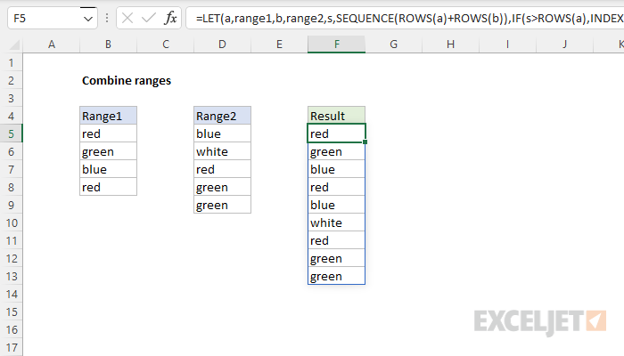
The formula to combine single column ranges is based on INDEX function , the SEQUENCE function , the IF function , and the LET function . In the example above, the formula in cell F5 is:
=LET(a,range1,b,range2,s,SEQUENCE(ROWS(a)+ROWS(b)),IF(s>ROWS(a),INDEX(b,s-ROWS(a)),INDEX(a,s)))
Adding line breaks to make the formula more readable, we have:
=LET(
   a,range1,
   b,range2,
   s,SEQUENCE(ROWS(a)+ROWS(b)),
   IF(s>ROWS(a),
      INDEX(b,s-ROWS(a)),
      INDEX(a,s)))
where range1 (B5:B8) and range2 (D5:D9) are named ranges . The first two lines inside let assign range1 to the variable “a” and assign range2 to the variable “b”.
Note: Range1 and Range2 do not have to be provided as named ranges; you could instead use B5:B8 and D5:D9.
Next, the SEQUENCE function creates a numeric “row index” to cover all rows in both ranges:
=SEQUENCE(ROWS(a)+ROWS(b))
=SEQUENCE(9)
={1;2;3;4;5;6;7;8;9}
The resulting array is assigned to the variable “s”. In the next line, the IF function is used to iterate through the array. If the current value s is greater than the rows in a , the INDEX function returns the value of b at row s minus the row count of a :
INDEX(b,s-ROWS(a)) // value from b
Otherwise, the INDEX function returns the value of a at row s :
INDEX(a,s) // value from a
The resulting values spill into the range F5:F13.
Note: a reader mentioned this formula to me based on the stackoverflow answer here .
Multiple column ranges
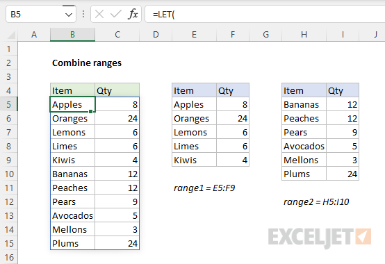
The formula to combine ranges with multiple columns is more complex. In the worksheet below, the formula in B5 looks like this
=LET(
   a,range1,
   b,range2,
   r,SEQUENCE(ROWS(a)+ROWS(b)),
   c,SEQUENCE(1,COLUMNS(a)),
   IF(
      r<=ROWS(a),
      INDEX(a,r,c),
      INDEX(b,r-ROWS(a),c))
)
where range1 (E5:F9) and range2 (H5:I10) are named ranges . Note that line breaks have been added for readability.
Like the formula above, this formula figures out how many rows are in both ranges, and uses the SEQUENCE function to create a “row index” with the SEQUENCE function here:
SEQUENCE(ROWS(a)+ROWS(b)) // returns {1;2;3;4;5;6;7;8;9;10;11}
In a similar way, SEQUENCE is also used to create a “column index”, named “c”:
SEQUENCE(1,COLUMNS(a)) // returns {1,2}
The IF function tests all values in the row index sequence with the row count for range 1. When a row index value is less than or equal to the count of the rows in a (5), the INDEX function is used to fetch a row from range a at the current index value (r) :
INDEX(a,r,c) // from range a
When a row index value is greater than 5, INDEX is used to fetch rows from b :
INDEX(b,r-ROWS(a),c))
Note c remains constant as {1,2} , the column index for range a . This is a shortcut to keep things simple. This formula does not try to figure out if the column counts for both ranges are the same or not. It simply assumes the column counts are the same and requests both columns.
Custom function with LAMBDA
The LAMBDA function can be used to create custom functions. The formula on this page is a good candidate, because it is relatively complex. When converted to a custom LAMBDA function, it is much easier to call:
=AppendRange(range1,range2)
See this article for more detail.
Explanation
In this example, the goal is to count the unique dates in a range of timestamps (i.e. dates that contain dates and times). In addition, we also want to create the table of results seen in E7:F9. For convenience, data is the named range B5:B16.
Basic count
To get a count of individual dates that occur in B5:B16, ignoring time values, the formula in F4 is:
=COUNT(UNIQUE(INT(data)))
Working from the inside out, the INT function is used to remove the time values from the timestamps like this:
INT(data) // remove time
This works because Excel dates are just serial numbers and Excel times are fractional dates that appear as decimal values. The INT function simply removes the decimal portion of the date, leaving the serial number intact. Because we are giving the INT function 12 separate values, INT returns 12 results in an array like this:
{44600;44600;44600;44600;44604;44604;44604;44635;44635;44635;44635;44635}
Each serial number in this array represents a date in data . Next, the UNIQUE function is used to remove duplicate dates. The two functions work together like this:
UNIQUE(INT(data)) // returns {44600;44604;44635}
Because there are 3 unique dates, UNIQUE returns 3 serial numbers in an array like this:
{44600;44604;44635}
This array is delivered directly to the COUNT function:
=COUNT({44600;44604;44635}) // returns 3
and the COUNT function (which counts numbers only) returns 3 as a final result.
Summary table in two parts
An easy way to create the summary table seen in the worksheet is to use two formulas. To list the 3 unique dates starting in cell D7, you can use:
=UNIQUE(INT(data)) // unique dates
To count how many times each date occurs in the data, you can enter this formula in cell F7 and copy it down:
=SUM(--(INT(data)=K7))
Note: we can’t use the COUNTIF function in this case (which would be easier) because we don’t have the dates without times in an actual range . Instead, the dates exist in an array returned by the INT function. COUNTIF requires a range for the range argument.
All-in-one summary table
To create an all-in-one summary table that lists the unique dates along with a count for each date, you can use an advanced formula like this:
=LET(d,INT(data),u,UNIQUE(d),HSTACK(u,SCAN(0,u,LAMBDA(a,v,SUM(--(v=d))))))
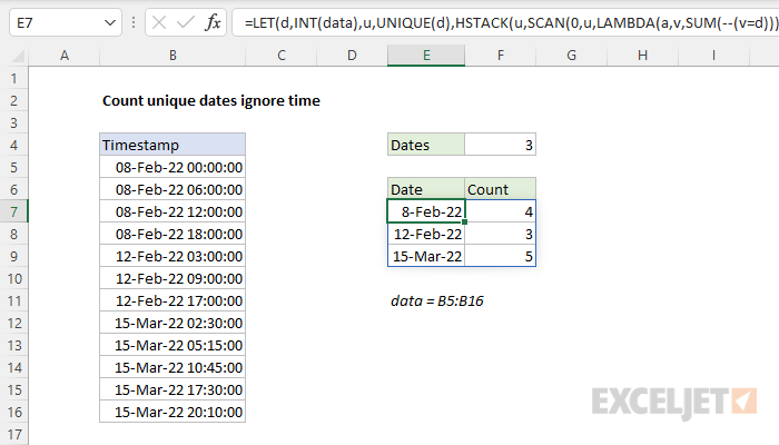
The LET function is used to assign intermediate results to named variables. First, we use INT to strip times from dates and assign the result to d . Then we feed d into UNIQUE (to get unique dates) and assign the result to u. Next, we use the HSTACK function to combine two arrays. Array1 is u (the unique dates), and array2 is generated with the SCAN function :
SCAN(0,u,LAMBDA(a,v,SUM(--(v=d))))
With an initial value of zero, SCAN iterates through each date in u and runs a custom LAMBDA function to count how many times the date appears in d :
LAMBDA(a,v,SUM(--(v=d))
The count is generated with boolean logic and the SUM function . The result from SCAN is an array with 3 counts:
{4;3;5}
This array is returned to HSTACK as array2 . HSTACK joins array1 and array2 together horizontally, and returns the 2-column array as a final result.
