Explanation
When conditional formatting is applied with a formula, the formula is evaluated relative to the active cell in the selection at the time the rule is created. In this case, the active cell when the rule is created is assumed to be cell E5, with the range E5:E14 selected.
As the formula is evaluated, formula references change so that the rule is testing for blank values in the correct row for each of the 10 cells in the range:
=OR(B5="",C5="", D5="") // E5
=OR(B6="",C6="", D6="") // E6
=OR(B7="",C7="", D7="") // E7
etc.
If any cell in a corresponding row in column B, C, or D is blank, OR function returns TRUE and the rule is triggered and the green fill is applied. When all tests return FALSE, the OR function returns FALSE and no conditional formatting is applied.
With ISBLANK
of testing for an empty string (="") directly you can use the ISBLANK function in an equivalent formula like this:
=OR(ISBLANK(B5),ISBLANK(C5),ISBLANK(D5))
AND, OR, NOT
Other logical tests can be constructed using combinations of AND, OR, and NOT. For example, to test for a blank cell in column B and column D, you could use a formula like this:
=AND(B5="",D5="")
This will trigger conditional formatting only when the column B and D are blank.
For more information on building formula criteria, see 50+ formula criteria examples .
Explanation
In this example, we want to apply three different colors, depending on how much the original date varies from the current date:
- Green if the variance is less than 3 days
- Yellow if the variance is between 3 and 10 days
- Red if the variance is greater than 10 days
For each rule, we calculate a variance by subtracting the original date from the “current” date (as explained above). Then we check the result with a logical expression. When an expression returns TRUE, the conditional formatting is triggered.
Because we want three separate colors, each with a logical test, we’ll need three separate conditional formatting rules. The screen below shows how the rules have been configured to apply the green, yellow, and red formatting. Note the first two rules have “stop if true” ticked:
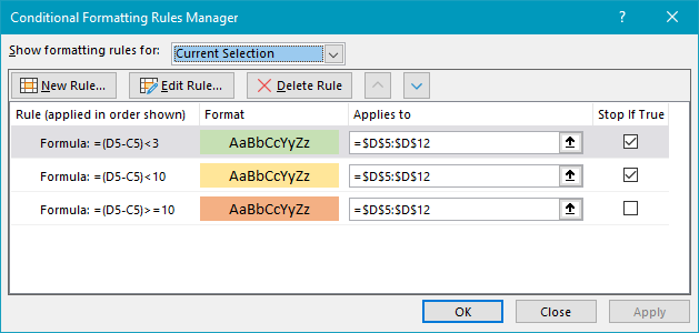
Rules are evaluated in the order shown. Rule 1 tests if the variance is less than 3 days. Rule 2 checks if the variance is less than 10 days. Rule 3 checks if the variance is greater than or equal to 10 days. Both rule 1 and rule 2 have “stop if true” enabled. When either rule returns TRUE, Excel will stop checking additional rules.
Overdue by n days from today
You might want to compare a due date to today’s date. To test if dates are overdue by at least n days from today, you can use a formula like this:
=(TODAY()-date)>=n
This formula will return TRUE only when a date is at least n days in the past. When a date is in the future, the difference will be a negative number, so the rule will never fire.
For more information on building formula criteria, see 50+ formula criteria examples .
