Explanation
Conditional formatting rules are evaluated in order.
- For each cell in the range B5:B12, the first formula is evaluated. If the value is greater than or equal to 90%, the formula returns TRUE and the green fill is applied. If the value is not greater than or equal to 90%, the formula returns FALSE and the rule is not triggered.
- For each cell in the range B5:B12, the second formula is evaluated. If the value is greater than or equal to 80%, the formula returns TRUE and the yellow fill is applied.
- For each cell in the range B5:B12, the third formula is evaluated. If the value is less than 80%, the formula returns TRUE and the pink fill is applied.
The “stop if true” option is enabled for the first two rules to prevent further processing, since the rules are mutually exclusive.
Explanation
This example is based on the formula explained in detail here :
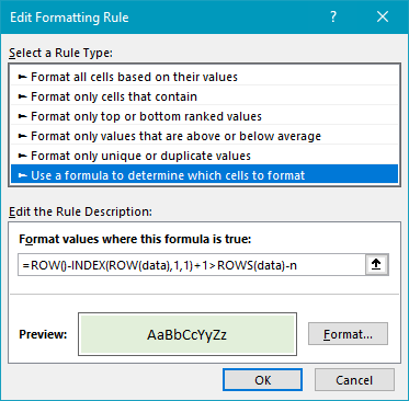
=ROW()-INDEX(ROW(data),1,1)+1>ROWS(data)-n
The formula uses the greater than operator (>) to check row in the data. On the left, the formula calculates a “current row”, normalized to begin at the number 1:
=ROW()-INDEX(ROW(data),1,1)+1 // calculate current row
On the right, the formula generates a threshold number:
ROWS(data)-n // calculate threshold
When the current row is greater than the threshold, the formula returns TRUE, triggering the conditional formatting.
Conditional formatting rule
The conditional formatting rule is set up to use a formula like this:
With a table
You can’t use a table name in a CF formula at present . However, you can select or enter the table data range when creating the formula in the CF window, and Excel will keep the reference up to date as the table expands or shrinks.
