Conditional Formatting With Formulas

Quick Links

Quick Start
Examples
Troubleshooting
Training

Conditional formatting is a fantastic way to quickly visualize data in a spreadsheet. With conditional formatting, you can do things like highlight dates in the next 30 days, flag data entry problems, highlight rows that contain top customers, show duplicates, and more.

Excel ships with a large number of “presets” that make it easy to create new rules without formulas. However, you can also create rules with your own custom formulas. By using your own formula, you take over the condition that triggers a rule and can apply exactly the logic you need. Formulas give you maximum power and flexibility.

For example, using the “Equal to” preset, it’s easy to highlight cells equal to “apple”.

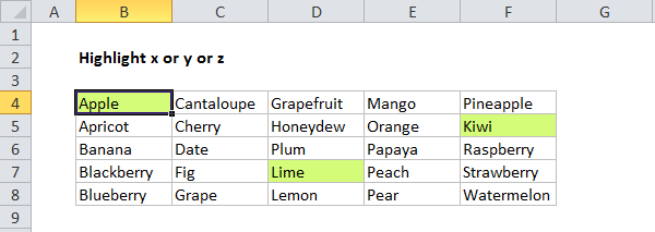
But what if you want to highlight cells equal to “apple” or “kiwi” or “lime”? Sure, you can create a rule for each value, but that’s a lot of trouble. Instead, you can simply use one rule based on a formula with the OR function :

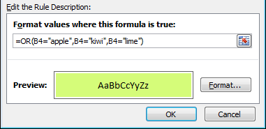
Here’s the result of the rule applied to the range B4:F8 in this spreadsheet:

Conditional formatting with the OR function - 2

Here’s the exact formula used:

=OR(B4="apple",B4="kiwi",B4="lime")

Quick start

You can create a formula-based conditional formatting rule in four easy steps:

Select the cells you want to format.

Create a conditional formatting rule, and select the Formula option

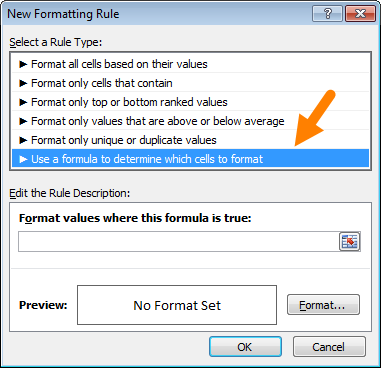
Enter a formula that returns TRUE or FALSE.

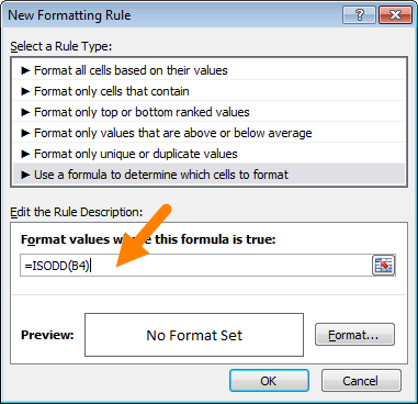
Enter the formula relative to the active cell - 5

Set formatting options and save the rule.

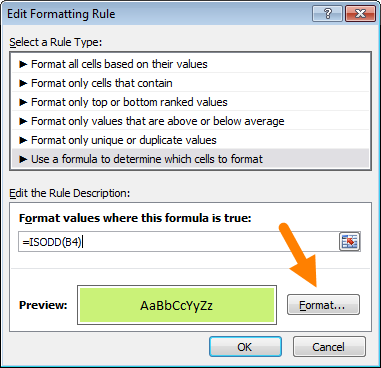
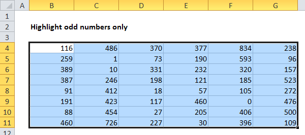
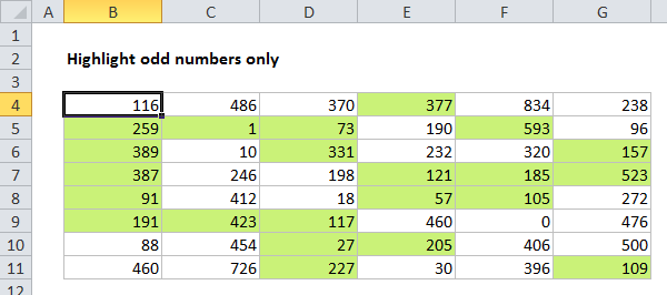
The ISODD function only returns TRUE for odd numbers, triggering the rule:

The ISODD function returns TRUE for odd numbers, triggering the rule - 7

Video: How to apply conditional formatting with a formula

We also offer video training on conditional formatting .

Formula logic

Formulas that apply conditional formatting must return TRUE or FALSE, or numeric equivalents. Here are some examples:

=ISODD(A1)
=ISNUMBER(A1)
=A1>100
=AND(A1>100,B1<50)
=OR(F1="MN",F1="WI")

The above formulas all return TRUE or FALSE, so they work perfectly as a trigger for conditional formatting.

When conditional formatting is applied to a range of cells, enter cell references with respect to the upper-left cell. The trick to understanding how conditional formatting formulas work is to visualize the same formula being applied to each cell in the selection , with cell references updated as usual. Imagine that you entered the formula in the upper-left cell of the selection, and then copied the formula across the entire selection. If you struggle with this, see the section on Dummy Formulas below.

Formula Examples

Below are examples of custom formulas you can use to apply conditional formatting. Some of these examples can be created using Excel’s built-in presets for highlighting cells, but custom formulas can go far beyond presets, as you can see below.

Also see: More than 30 Conditional Formatting Formulas

Highlight orders from Texas

To highlight rows that represent orders from Texas (abbreviated TX), use a formula that locks the reference to column F:

=$F5="TX"

For more details, see this article: Highlight rows with conditional formatting .

Video: How to highlight rows with conditional formatting

Highlight dates in the next 30 days

To highlight dates occurring in the next 30 days, we need a formula that (1) makes sure dates are in the future and (2) makes sure dates are 30 days or less from today. One way to do this is to use the AND function together with the NOW function like this:

=AND(B4>NOW(),B4<=(NOW()+30))

With a current date of August 18, 2016, the conditional formatting highlights dates as follows:

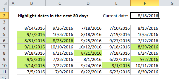
Conditional formatting to highlight dates in the next 30 days - 9

The NOW function returns the current date and time. For details about how this formula, works, see this article: Highlight dates in the next N days .

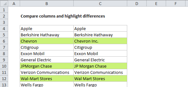
Highlight column differences

Given two columns that contain similar information, you can use conditional formatting to spot subtle differences. The formula used to trigger the formatting below is:

=$B4<>$C4

Conditional formatting to compare columns - 10

Highlight missing values

To highlight values in one list that are missing from another, you can use a formula based on the COUNTIF function :

=COUNTIF(list,B5)=0

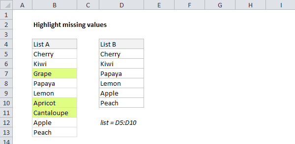
Highlight missing values with conditional formatting - 11

This formula simply checks each value in List A against values in the named range “list” (D5:D10). When the count is zero, the formula returns TRUE and triggers the rule, which highlights values in List A that are missing from List B .

Video: How to find missing values with COUNTIF

Highlight properties with 3+ bedrooms under $350k

To find properties in this list that have at least 3 bedrooms but are less than $300,000, you can use a formula based on the AND function:

=AND($C5<350000,$D5>=3)

The dollar signs ($) lock the reference to columns C and D, and the AND function is used to make sure both conditions are TRUE. In rows where the AND function returns TRUE, the conditional formatting is applied:

Conditional formatting to highlight property listings - 12

Highlight top values (dynamic example)

Although Excel has presets for “top values”, this example shows how to do the same thing with a formula, and how formulas can be more flexible. By using a formula, we can make the worksheet interactive — when the value in F2 is updated, the rule instantly responds and highlights new values.

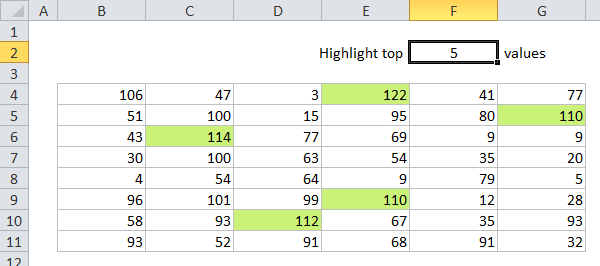
Dynamic conditional formatting for top values - 13

The formula used for this rule is:

=B4>=LARGE(data,input)

Where “data” is the named range B4:G11, and “input” is the named range F2. This page has details and a full explanation .

Gantt charts

Believe it or not, you can even use formulas to create simple Gantt charts with conditional formatting like this:

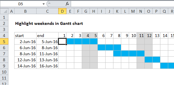
Using conditional formatting to create a Gantt chart - 14

This worksheet uses two rules, one for the bars, and one for the weekend shading:

=AND(D$4>=$B5,D$4<=$C5) // bars
=WEEKDAY(D$4,2)>5 // weekends

This article explains the formula for bars , and this article explains the formula for weekend shading .

One cool trick you can do with conditional formatting is to build a simple search box. In this example, a rule highlights cells in column B that contain text typed in cell F2:

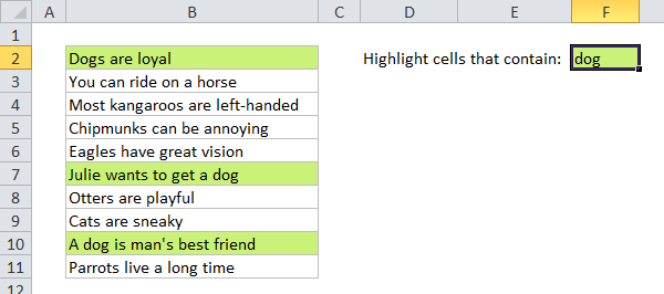
The formula used is:

=ISNUMBER(SEARCH($F$2,B2))

For more details and a full explanation, see:

Article: How to highlight cells that contain specific text
Article: How to highlight rows that contain specific text
Video: How to build a search box to highlight data

Troubleshooting

If you can’t get your conditional formatting rules to fire correctly, there’s most likely a problem with your formula. First, make sure you started the formula with an equals sign (=). If you forget this step, Excel will silently convert your entire formula to text, rendering it useless. To fix, just remove the double quotes Excel added at either side and make sure the formula begins with equals (=).

If your formula is entered correctly but is not triggering the rule, you may have to dig a little deeper. Normally, you can use the F9 key to check results in a formula or use the Evaluate feature to step through a formula. Unfortunately, you can’t use these tools with conditional formatting formulas, but you can use a technique called “dummy formulas”.

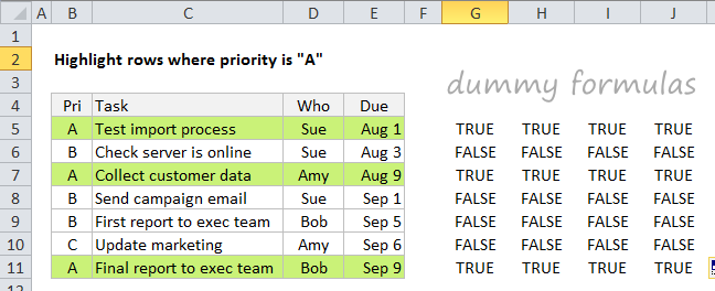
Dummy Formulas

Dummy formulas are a way to test your conditional formatting formulas directly on the worksheet, so you can see what they’re actually doing. This can be a big time-saver when you’re struggling to get cell references working correctly.

In a nutshell, you enter the same formula across a range of cells that matches the shape of your data. This lets you see the values returned by each formula, and it’s a great way to visualize and understand how formula-based conditional formatting works. For a detailed explanation, see this article .

Use dummy formulas to check conditional formatting formulas - 16

Video: Test conditional formatting with dummy formulas

Limitations

There are some limitations that come with formula-based conditional formatting:

You can’t apply icons, color scales, or data bars with a custom formula. You are limited to standard cell formatting, including number formats, font, fill color, and border options.
You can’t use certain formula constructs like unions, intersections, or array constants for conditional formatting criteria.
You can’t reference other workbooks in a conditional formatting formula.

You can sometimes work around #2 and #3. You may be able to move the logic of the formula into a cell in the worksheet, and then refer to that cell in the formula instead. If you are trying to use an array constant, try creating a named range instead.

More CF formula resources

More than 30 conditional formatting formulas examples
Video training with practice worksheets

The IF function is one of the most heavily used functions in Excel. IF is a simple function, and people love IF because it gives them the power to make Excel respond as information is entered in a spreadsheet. With IF, you can bring your spreadsheet to life.

But one IF often leads to another, and once you combine more than a couple IFs, your formulas can start to look like little Frankensteins :)

Are nested IFs evil? Are they sometimes necessary? What are the alternatives?

Read on to learn the answers to these questions and more…

1. Basic IF

Before we talk about nested IF, let’s quickly review the basic IF structure:

=IF(test,[true],[false])

The IF function runs a test and performs different actions depending on whether the result is true or false.

Note the square brackets…these mean the arguments are optional. However, you must supply either a value for true, or a value for false.

To illustrate, here we use IF to check scores and calculate “Pass” for scores of at least 65:

Cell D3 in the example contains this formula:

=IF(C3>=65,"Pass")

Translation: if the score in C3 is at least 65, return “Pass”.

Note however that if the score is less than 65, IF returns FALSE, since we didn’t supply a value if false. To display “Fail” for non-passing scores, we can add “Fail” as the false argument like so:

=IF(C3>=65,"Pass","Fail")

Basic IF function - with a value added for false - 18

Video: How to build logical formulas .

2. What nesting means

Nesting simply means to combine formulas, one inside the other, so that one formula handles the result of another. For example, here’s a formula where the TODAY function is nested inside the MONTH function:

=MONTH(TODAY())

The TODAY function returns the current date inside of the MONTH function. The MONTH function takes that date and returns the current month. Even moderately complex formulas use nesting frequently, so you’ll see nesting everywhere in more complex formulas.

3. A simple nested IF

A nested IF is just two more IF statements in a formula, where one IF statement appears inside the other.

To illustrate, below I’ve extended the original pass/fail formula above to handle “incomplete” results by adding an IF function, and nesting one IF inside the other:

=IF(C3="","Incomplete",IF(C3>=65,"Pass","Fail"))

The outer IF runs first and tests to see if C3 is blank. If so, outer IF returns “Incomplete”, and the inner IF never runs.

If the score is not blank , the outer IF returns FALSE, and the original IF function is run.

Learn nested IFs with clear, concise video training .

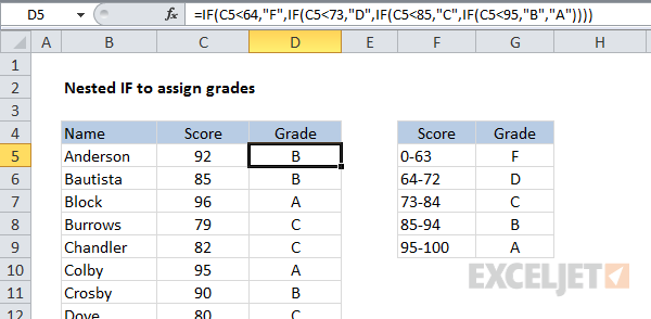
4. A nested IF for scales

You’ll often see nested IFs set up to handle “scales”…for example, to assign grades, shipping costs, tax rates, or other values that vary on a scale with a numerical input. As long as there aren’t too many levels in the scale, nested IFs work fine here, but you must keep the formula organized, or it becomes difficult to read.

The trick is to decide a direction (high to low, or low to high), then structure the conditions accordingly. For example, to assign grades in a “low to high” order, we can represent the solution needed in the following table. Note there is no condition for “A”, because once we’ve run through all the other conditions, we know the score must be greater than 95, and therefore an “A”.

Score	Grade	Condition
0-63	F	<64
64-72	D	<73
73-84	C	<85
85-94	B	<95
95-100	A

With the conditions clearly understood, we can enter the first IF statement:

=IF(C5<64,"F")

This takes care of “F”. Now, to handle “D”, we need to add another condition:

=IF(C5<64,"F",IF(C5<73,"D"))

Note that I simply dropped another IF into the first IF for the “false” result. To extend the formula to handle “C”, we repeat the process:

=IF(C5<64,"F",IF(C5<73,"D",IF(C5<85,"C")))

We continue on this way until we reach the last grade. Then, instead of adding another IF, just add the final grade for false.

=IF(C5<64,"F",IF(C5<73,"D",IF(C5<85,"C",IF(C5<95,"B","A"))))

Here is the final nested IF formula in action:

Completed nested IF example for calculating grades - 20

Video: How to make a nested IF to assign grades

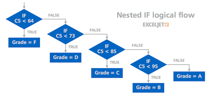
5. Nested IFs have a logical flow

Many formulas are solved from the inside out, because “inner” functions or expressions must be solved first for the rest of the formula to continue.

Nested IFs have their own logical flow, where the “outer” IFs act like a gateway to “inner” IFs. This means that results from outer IFs determine whether inner IFs even run. The diagram below visualizes the logical flow of the grade formula above.

6. Use Evaluate to watch the logical flow

On Windows, you can use the Evaluate feature to watch Excel solve your formulas, step-by-step. This is a great way to “see” the logical flow of more complex formulas and to troubleshoot when things aren’t working as you expect. The screen below shows the Evaluate window open and ready to go. Each time you click the Evaluate button, the “next step” in the formula is solved. You can find Evaluate on the Formulas tab of the ribbon (Alt M, V).

Using Evaluate to step through a nested IF that assigns grades - 22

Unfortunately, the Mac version of Excel doesn’t contain the Evaluate feature, but you can still use the F9 trick below.

7. Use F9 to spot-check results

When you select an expression in the formula bar and press the F9 key, Excel solves just the part selected. This is a powerful way to confirm what a formula is really doing. In the screen below, I am using the screen tip windows to select different parts of the formula, then clicking F9 to see that part solved:

Using F9 check a nested IF that assigns grades - 23

Use Control + Z (Command + Z) on a Mac to undo F9. You can also press Esc to exit the formula editor without any changes.

Video: How to debug a formula with F9

8. Know your limits

Excel has limits on how deeply you can nest IF functions. Up to Excel 2007, Excel allowed up to 7 levels of nested IFs. In Excel 2007+, Excel allows up to 64 levels.

However, just because you can nest a lot of IFs, it doesn’t mean you should . Every additional level you add makes the formula more difficult to understand and troubleshoot. If you find yourself working with a nested IF more than a few levels deep, you should probably take a different approach — see the below for alternatives.

9. Match parentheses like a pro

One of the challenges with nested IFs is matching or “balancing” parentheses. When parentheses aren’t matched correctly, your formula is broken. Luckily, Excel provides a couple of tools to help you make sure parentheses are “balanced” while editing formulas.

First, once you have more than one set of parentheses, the parentheses are color-coded so that opening parentheses match closing parentheses. These colors are pretty darn hard to see, but they are there if you look closely:

Formula parentheses are color-matched but hard to see - 24

Second (and better) when you close parentheses, Excel will briefly bold the matching pair. You can also click into the formula and use the arrow key to move through parentheses, and Excel will briefly bold both parentheses when there is a matching pair. If there is no match, you’ll see no bolding.

Unfortunately, the bolding is a Windows-only feature. If you’re using Excel on a Mac to edit complex formulas, it sometimes makes sense to copy and paste the formula into a good text editor ( Text Wrangler is free and excellent) to get better parentheses-matching tools. Text Wrangler will flash when parentheses are matched, and you can use Command + B to select all text contained by parentheses. You can paste the formula back into Excel after you’ve straightened things out.

10. Use the screen tip window to navigate and select

When it comes to navigating and editing nested IFs, the function screen tip is your best friend. With it, you can navigate and precisely select all arguments in a nested IF:

Navigate and select formula arguments with the screen tip - 25

You can see me use the screen tip window a lot in this video: How to build a nested IF .

11. Take care with text and numbers

Just as a quick reminder, when working with the IF function, take care that you a properly handling numbers and text. For example, I often see formulas like this:

=IF(A1="100","Pass","Fail")

Is the test score in A1 really text and not a number? No? Then don’t use quotes around the number. Otherwise, the logical test will never return FALSE even when the value is a passing score, because “100” is not the same as 100. If the test score is numeric, use this:

=IF(A1=100,"Pass","Fail")

12. Add line breaks to make nested IFs easy to read

When you’re working with a formula that contains many levels of nested IFs, it can be tricky to keep things straight. Because Excel doesn’t care about “white space” in formulas (i.e. extra spaces or line breaks), you can greatly improve the readability of nested ifs by adding line breaks.

For example, the screen below shows a nested IF that calculates a commission rate based on a sales number. Here you can see the typical nested IF structure, which is hard to decipher:

Nested IFs without line breaks are difficult to read - 26

However, if I add line breaks before each “value if false”, the logic of the formula jumps out clearly. Plus, the formula is easier to edit:

Line breaks make nested IFs easier to read - 27

You can add line breaks on Windows with Alt + Enter, on a Mac, use Control + Option + Return.

Video: How to make a nested IF easier to read .

13. Limit IFs with AND and OR

Nested IFs are powerful, but they become complicated quickly as you add more levels. One way to avoid more levels is to use IF in combination with the AND and OR functions. These functions return a simple TRUE/FALSE result that works perfectly inside IF, so you can use them to extend the logic of a single IF.

For example, in the problem below, we want to put an “x” in column D to mark rows where the color is “red” and the size is “small”.

IF with the AND function is simpler than two nested IFs - 28

We could write the formula with two nested IFs like this:

=IF(B6="red",IF(C6="small","x",""),"")

However, by replacing the test with the AND function, we can simplify the formula:

=IF(AND(B6="red",C6="small"),"x","")

In the same way, we can easily extend this formula with the OR function to check for red OR blue AND small:

=IF(AND(OR(B4="red",B4="blue"),C4="small"),"x","")

All of this could be done with nested IFs, but the formula would rapidly become more complex.

Video: IF this OR that

14. Replace Nested IFs with VLOOKUP

When a nested IF is simply assigning values based on a single input, it can be easily replaced with the VLOOKUP function . For example, this nested IF assigns numbers to five different colors:

=IF(E3="red",100,IF(E3="blue",200,IF(E3="green",300,IF(E3="orange",400,500))))

We can easily replace it with this (much simpler) VLOOKUP:

=VLOOKUP(E3,B3:C7,2,0)

As a bonus, VLOOKUP keeps values on the worksheet (where they can be easily changed) instead of embedding them in the formula.

Although the formula above uses exact matching, you can easily use VLOOKUP for grades as well.

Video: How to use VLOOKUP

Video: Why VLOOKUP is better than nested IFs

15. Choose CHOOSE

The CHOOSE function can provide an elegant solution when you need to map simple, consecutive numbers (1,2,3, etc.) to arbitrary values.

In the example below, CHOOSE is used to create custom weekday abbreviations:

Sure, you could use a long and complicated nested IF to do the same thing, but please don’t :)

16. Use IFS instead of nested IFs

In more recent versions of Excel there is a new function you can use instead of nested IFs: the IFS function . The IFS function provides a special structure for evaluating multiple conditions without nesting:

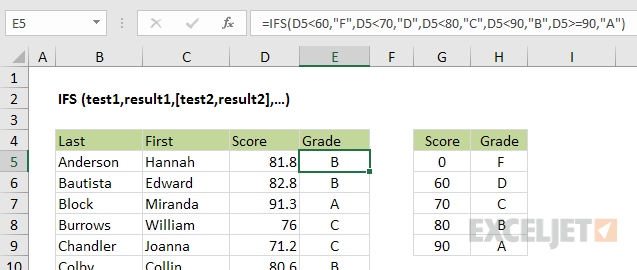
The IFS function - multiple conditions without nesting - 31

The formula used above looks like this:

=IFS(D5<60,"F",D5<70,"D",D5<80,"C",D5<90,"B",D5>=90,"A")

Note we have just a single pair of parentheses since all conditions are handled as separate arguments the IFS function.

17. Max out

Sometimes, you can use MAX or MIN in a very clever way that avoids an IF statement. For example, suppose you have a calculation that needs to result in a positive number, or zero. In other words, if the calculation returns a negative number, you just want to show zero.

The MAX function gives you a clever way to do this without an IF anywhere in sight:

=MAX(calculation,0)

This technique returns the result of the calculation if positive, and zero otherwise.

I love this construction because its just so simple . See this article for a full write-up .

18. Trap errors with IFERROR

A classic use of IF is to trap errors and supply another result when an error is thrown, like this:

=IF(ISERROR(formula),error_result,formula)

This is ugly and redundant, since same formula goes in twice, and Excel has to calculate the same result twice when there is no error.

In Excel 2007, the IFERROR function was introduced, which lets you trap errors much more elegantly:

=IFERROR(formula,error_result)

Now when the formula throws an error, IFERROR simply returns the value you provide.

19. Use boolean logic

You can also sometimes avoid nested IFs by using what’s called “boolean logic”. The word boolean refers to TRUE/FALSE values. Although Excel displays the words TRUE and FALSE in cells, internally, Excel treats TRUE as 1 and FALSE as zero. You can use this fact to write clever, and very fast formulas. For example, in the VLOOKUP example above, we have a nested IF formula that looks like this:

=IF(E3="red",100,IF(E3="blue",200,IF(E3="green",300,IF(E3="orange",400,500))))

Using boolean logic, you can rewrite the formula like this:

=(E3="red")*100+(E3="blue")*200+(E3="green")*300+(E3="orange")*400+(E3="purple")*500

Each expression performs a test, and then multiples the outcome of the test by the “value if true”. Since tests return either TRUE or FALSE (1 or 0), the FALSE results effectively cancel themselves out of the formula.

For numeric results, boolean logic is simple and extremely fast, since there is no branching. On the downside, boolean logic can be confusing to people who aren’t used to seeing it. Still, it’s a great technique to know about.

Video: How to use boolean logic in Excel formulas

When do you need a nested IF?

With all these options for avoiding nested IFs, you might wonder when it makes sense to use a nested IF?

I think nested IFs make sense when you need to evaluate several different inputs to make a decision.

For example, suppose you want to calculate an invoice status of “Paid”, “Open”, “Overdue”, etc. This requires that you look at the invoice age and outstanding balance:

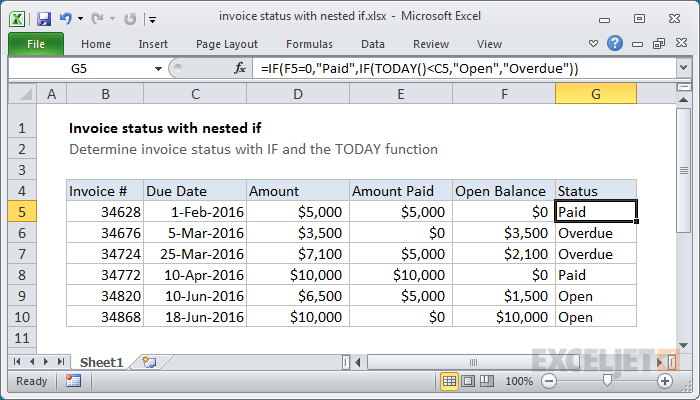
Calculating invoice status with a nested IF - 32

In this case, a nested IF is a perfectly fine solution.

Your thoughts?

What about you? Are you an IF-ster? Do you avoid nested IFs? Are nested IFs evil? Share your thoughts below.

Learn Excel formulas quickly with concise video training .

Quick Links#

Quick start#

Formula logic#

Formula Examples#

Highlight orders from Texas#

Highlight dates in the next 30 days#

Highlight column differences#

Highlight missing values#

Highlight properties with 3+ bedrooms under $350k#

Highlight top values (dynamic example)#

Gantt charts#

Simple search box#

Troubleshooting#

Dummy Formulas#

Limitations#

More CF formula resources#

1. Basic IF#

2. What nesting means#

3. A simple nested IF#

4. A nested IF for scales#

5. Nested IFs have a logical flow#

6. Use Evaluate to watch the logical flow#

7. Use F9 to spot-check results#

8. Know your limits#

9. Match parentheses like a pro#

10. Use the screen tip window to navigate and select#

11. Take care with text and numbers#

12. Add line breaks to make nested IFs easy to read#

13. Limit IFs with AND and OR#

14. Replace Nested IFs with VLOOKUP#

15. Choose CHOOSE#

16. Use IFS instead of nested IFs#

17. Max out#

18. Trap errors with IFERROR#

19. Use boolean logic#

When do you need a nested IF?#

Your thoughts?#