Explanation
To convert an expense in one time unit (i.e. daily, weekly, monthly, etc.) to other time units, you can use a two-way INDEX and MATCH formula. In the example shown, the formula in E5 (copied across and down) is :
=$C5*INDEX(data,MATCH($D5,vunits,0),MATCH(F$4,hunits,0))
This formula uses a lookup table with named ranges as shown below:
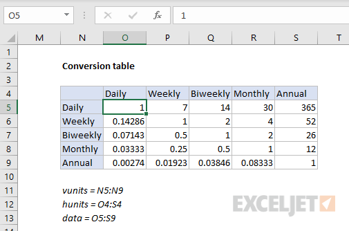
Named ranges: data (O5:S9), vunits (N5:N9), and hunits (O4:S4).
Introduction
The goal is to convert an expense in one time unit, to an equivalent expense in other time units. For example, if we have a monthly expense of $30, we want to calculate an annual expense of $360, a weekly expense of $7.50, etc.
Like so many challenges in Excel, much depends on how you approach the problem. You might first be tempted to consider a chain of nested IF formulas. This can be done, but you’ll end up with a long and complicated formula.
A cleaner approach is to build a lookup table that contains conversion factors for all possible conversions, then use a two-way INDEX and MATCH formula to retrieve the required value for a given conversion. Once you have the value, you can simply multiply by the original amount.
The conversion table
The conversion table has the same values for both vertical and horizontal labels: daily, weekly, biweekly, monthly, and annual. The “from” units are listed vertically, and the “to” units are listed horizontally. For the purposes of this example, we want to match the row first, then the column. So, if we want to convert a monthly expense to an annual expense, we match the “monthly” row, and the “annual” column, and return 12.

To populate the table itself, we use a mix of simple formulas and constants:

Note: Customize conversion values to meet your specific needs. Entering a value as =1/7 is an easy way to avoid entering long decimal values.
The lookup formula
Since we need to locate a conversion value based on two inputs, a “from” time unit and a “to” time unit, we need a two-way lookup formula. INDEX and MATCH provides a nice solution. In the example shown, the formula in E5 is:
=$C5*INDEX(data,MATCH($D5,vunits,0),MATCH(F$4,hunits,0))
Working from the inside out, the first MATCH function locates the correct row:
MATCH($D5,vunits,0) // find row, returns 4
We pull the original “from” time unit from column D, which we use to find the right row in the named range vunits (N5:N9). Note $D5 is a mixed reference with the column locked, so the formula can be copied across.
The second MATCH function locates the column:
MATCH(F$4,hunits,0) // find column, returns 5
Here, we get the lookup value from the column header in row 4, and use this to find the right “to” column in the named range hunits (O4:S4). Again, note F$4 is a mixed reference with the row locked, so the formula can be copied down.
After both MATCH formulas return results to INDEX, we have:
=$C5*INDEX(data,4,5)
The array provided to INDEX is the named range data , (O5:S9). With a row of 4 and column of 5, INDEX returns 12, so we get a final result of 12000 like this:
=$C5*INDEX(data,4,5)
=1000*12
=12000
Explanation
In this example the goal is to parse feet and inches out in the text strings shown in column B, and create a single numeric value for total inches. The challenge is that each of the two numbers is embedded in text. The formula can be divided into two parts. In the first part of the formula, feet are extracted and converted to inches. In the second part, inches are extracted and added to the result.
Extracting feet
To extract feet and convert them to inches, we use the following snippet:
=LEFT(B5,FIND("'",B5)-1)*12
Working from the inside out, the FIND function is used to locate the position of the single quote (’) in the string:
FIND("'",B5) // returns 2
We then subtract 1 (-1) and feed the result into the LEFT function as the number of characters to extract from the left:
LEFT(B5,1) // returns "8"
For cell B5, LEFT returns “8,” which is then multiplied by 12 to get 96 inches. Note that the LEFT function will return a text value , but the math operation of multiplying by 12 will automatically convert the text to a number.
Extracting inches
In the second part of the formula, we extract the value for inches from the text with this snippet:
SUBSTITUTE(MID(B5,FIND("'",B5)+1,LEN(B5)),"""","")
Here we again locate the position of the single quote (’) in the string with FIND. This time, however, we add 1 (+1) so that we start extracting after the single quote:
FIND("'",B5)+1 // returns 3
The result is 3, which we feed into the MID function as the start number:
MID(B5,3,LEN(B5))
For the number of characters to extract, we cheat and use the LEN function . LEN will return the total characters in B5 (5), which is a larger number of characters than remain in the string. However, MID will simply extract all remaining characters without complaint:
MID(B5,3,5) // returns " 4"""
For B5, MID will return " 4""", which goes into the SUBSTITUTE function as text:
SUBSTITUTE(" 4""","""","") // returns " 4"
The SUBSTITUTE function is configured to replace the double quote (") character with an empty string (""). In B5, SUBSTITUTE returns " 4" as text. As before, the math operation of addition will convert text value (with a space) to a number automatically, and the formula in B5 will give a final result of 100. However, to guard against a hyphen, we hand off the number returned by SUBSTITUTE to the ABS function for reasons explained below.
Note: the use of four quote characters ("""") to refer to a single double quote character (") is somewhat confusing. In brief, the outer quotes indicate a text value, the second quote is an escape character, and the third quote is the actual value. More details here .
Handling the hyphen
The measurements in B12:B13, include a hyphen (-) between feet and inches. When a hyphen is present between feet and inches, it will cause Excel to interpret the inch value as a negative number and create an incorrect result, since inches will be subtracted instead of added. To guard against this problem, we hand off the number extracted for inches to the ABS function . For example, in B12, SUBSTITUTE returns “-3 1/2” and ABS returns 3.5:
ABS("-3 1/2") // returns 3.5
Using the ABS function this way allows the same formula to handle both cases. If a hyphen is present, ABS interprets the value as negative and flips the value to a positive number. If a hyphen is not present, ABS returns the number unchanged. ABS also coerces the text value to a number.
Other units
Once you have a numeric measurement in inches, you can use the CONVERT function to convert to other units of measure.
