Explanation
In this example the goal is to parse feet and inches out in the text strings shown in column B, and create a single numeric value for total inches. The challenge is that each of the two numbers is embedded in text. The formula can be divided into two parts. In the first part of the formula, feet are extracted and converted to inches. In the second part, inches are extracted and added to the result.
Extracting feet
To extract feet and convert them to inches, we use the following snippet:
=LEFT(B5,FIND("'",B5)-1)*12
Working from the inside out, the FIND function is used to locate the position of the single quote (’) in the string:
FIND("'",B5) // returns 2
We then subtract 1 (-1) and feed the result into the LEFT function as the number of characters to extract from the left:
LEFT(B5,1) // returns "8"
For cell B5, LEFT returns “8,” which is then multiplied by 12 to get 96 inches. Note that the LEFT function will return a text value , but the math operation of multiplying by 12 will automatically convert the text to a number.
Extracting inches
In the second part of the formula, we extract the value for inches from the text with this snippet:
SUBSTITUTE(MID(B5,FIND("'",B5)+1,LEN(B5)),"""","")
Here we again locate the position of the single quote (’) in the string with FIND. This time, however, we add 1 (+1) so that we start extracting after the single quote:
FIND("'",B5)+1 // returns 3
The result is 3, which we feed into the MID function as the start number:
MID(B5,3,LEN(B5))
For the number of characters to extract, we cheat and use the LEN function . LEN will return the total characters in B5 (5), which is a larger number of characters than remain in the string. However, MID will simply extract all remaining characters without complaint:
MID(B5,3,5) // returns " 4"""
For B5, MID will return " 4""", which goes into the SUBSTITUTE function as text:
SUBSTITUTE(" 4""","""","") // returns " 4"
The SUBSTITUTE function is configured to replace the double quote (") character with an empty string (""). In B5, SUBSTITUTE returns " 4" as text. As before, the math operation of addition will convert text value (with a space) to a number automatically, and the formula in B5 will give a final result of 100. However, to guard against a hyphen, we hand off the number returned by SUBSTITUTE to the ABS function for reasons explained below.
Note: the use of four quote characters ("""") to refer to a single double quote character (") is somewhat confusing. In brief, the outer quotes indicate a text value, the second quote is an escape character, and the third quote is the actual value. More details here .
Handling the hyphen
The measurements in B12:B13, include a hyphen (-) between feet and inches. When a hyphen is present between feet and inches, it will cause Excel to interpret the inch value as a negative number and create an incorrect result, since inches will be subtracted instead of added. To guard against this problem, we hand off the number extracted for inches to the ABS function . For example, in B12, SUBSTITUTE returns “-3 1/2” and ABS returns 3.5:
ABS("-3 1/2") // returns 3.5
Using the ABS function this way allows the same formula to handle both cases. If a hyphen is present, ABS interprets the value as negative and flips the value to a positive number. If a hyphen is not present, ABS returns the number unchanged. ABS also coerces the text value to a number.
Other units
Once you have a numeric measurement in inches, you can use the CONVERT function to convert to other units of measure.
Explanation
In this example, the goal is to create a formula that converts a numeric value in inches to a format that displays inches and feet, as seen in the table below:
| Input | Output |
|---|---|
| 9 | 0’ 9" |
| 12 | 1’ 0" |
| 30 | 2’ 6" |
| 75 | 6’ 3" |
The math for this problem is fairly simple, but the problem is more complex because we need to assemble a text string that includes a single quote for feet (’) and a double quote (") for inches. This means we need to concatenate numbers after we perform the necessary calculations. The article below explains a basic formula for positive inputs with several variations. It also includes an adjusted formula to handle negative inches and a more modern formula based on the LET function.
Basic formula
In the worksheet shown above, the formula in cell D5 looks like this:
=INT(B5/12)&"' "&MOD(B5,12)&""""
This formula converts a numeric value in inches to text representing the same measurement in inches and feet. To get a value for feet, the INT function is used like this:
=INT(B5/12) // get whole feet
Inside INT, the value in B5 is divided by 12. The INT function returns the integer portion of a decimal number and discards any decimal remainder. The result from INT is the number of whole feet in B5. To get a value for inches, we use the MOD function like this:
MOD(B5,12) // get inches
The MOD function divides B5 by 12 and returns the remainder, which corresponds to inches. At this point, we have a number for feet and a number for inches. The remaining task is to concatenate these numbers together into a text string that includes a single quote for feet (’) and a double quote (") for inches. We start by adding a single quote with a space to the value for feet:
=INT(B5/12)&"' "
We add a space to separate the feet from the inches. Then we insert another ampersand (&) and add the MOD part of the formula:
=INT(B5/12)&"' "&MOD(B5,12)
We finish with two sets of double quotes (""""):
=INT(B5/12)&"' "&MOD(B5,12)&""""
The outer pair of double quotes tells Excel this is a text value . The inner pair of quotes causes Excel to return one double quote ("). Finally, all values are concatenated together, and Excel returns a result.
Rounded inches
To round inches to a given number of decimal places, wrap the MOD function in the ROUND function . For example, to round inches to one decimal:
=INT(A1/12)&"' "&ROUND(MOD(A1,12),1)&""""
With complete labels
To output a value like “8 feet 4 inches”, you can adapt the formula like this:
=INT(B5/12)&" feet "&MOD(B5,12)&" inches"
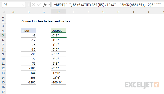
Negative numbers
We need a different formula to work with negative inches as an input. One solution is to use a formula like this:
=REPT("-",B5<0)&INT(ABS(B5)/12)&"' "&MOD(ABS(B5),12)&""""
This looks pretty complicated, but the core of this formula is almost the same as the original formula above. The difference is that we are using the ABS function to convert the input in cell B5 to a positive number. This needs to happen twice, each time we use B5:
=INT(ABS(B5)/12)&"' "&MOD(ABS(B5),12)&""""
After ABS runs, the formula works as before and returns a text string indicating feet and inches. The remaining step is to add a negative sign ("-") if the input is indeed negative. We do this with the REPT function at the start of the formula. REPT is designed to repeat text values by providing a number for the second argument, for example:
=REPT("A",1) // returns "A"
=REPT("A",2) // returns "AA"
=REPT("A",3) // returns "AAA"
In our formula, we use REPT in a tricky way like this:
=REPT("-",B5<0)
When B5 is less than zero, the result is TRUE, which evaluates to 1. When B5 is not less than zero, the result is FALSE, which evaluates to 0. The REPT function only returns “-” when the value is negative, otherwise it returns an empty string. Essentially, the REPT formula mimics this longer IF formula:
=IF(B5<0,"-","")
The final formula looks like this:
=REPT("-",B5<0)&INT(ABS(B5)/12)&"' "&MOD(ABS(B5),12)&""""
This formula will now correctly handle positive or negative input values.
Note: one reason we need to deal with negative numbers differently is that the INT function , contrary to its name, actually rounds negative numbers down away from zero. Another approach would be to switch to the TRUNC function , which just chops off the decimal value and keeps the integer with the sign. I tried that at first, but in the end I decided it made more sense to leave the original formula logic intact and treat the negative sign as a separate step.
LET formula option
A problem like this is a perfect candidate for the LET function , which makes it possible to assign variables inside a formula. Using LET, we can write an all-in-one formula like this:
=LET(
input,ABS(B5),
sign,IF(B5<0,"-",""),
feet,INT(input/12),
inches,MOD(input,12),
sign&feet&"' "&inches&"""")
This may look more complicated at first glance, but if you look closely, you will see that the first four lines create variables (input, sign, feet, inches) in a logical order. The last line concatenates the sign, feet, and inches together and returns the result. We only need to use the ABS function once. This formula will handle positive or negative inputs.
This version of the formula does not use the REPT trick for the sake of readability, but it could.
