Purpose
Return value
Syntax
=CORREL(array1,array2)
- array1 - The first set of data values.
- array2 - The second set of data values.
Using the CORREL function
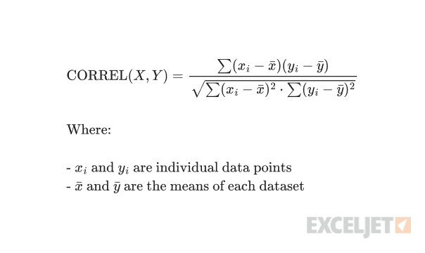
The CORREL function calculates the Pearson correlation coefficient between two data sets. It measures both the strength and direction of the linear relationship between variables, providing a standardized measure that ranges from -1 to 1.
Key features
- Returns values between -1 and 1 (inclusive)
- Positive values close to 1 indicate positive correlation
- Negative values close to -1 indicate negative correlation
- Values close to zero indicate weak correlation
- Unit-independent and standardized measure
- Both arrays must have the same number of data points
- Works with numbers only - text and logical values are ignored
Note: Excel also provides PEARSON function which is identical to CORREL. Both calculate the Pearson product-moment correlation coefficient.
- Example #1 - Strong Positive Correlation
- Example #2 - Strong Negative Correlation
- Example #3 - Weak Correlation
- When to use CORREL
- Formula Definition
- Notes
Example #1 - Strong Positive Correlation
In this example, we’ll examine the relationship between temperature (°F) and ice cream sales ($). As temperature increases, ice cream sales tend to increase as well, demonstrating a strong positive correlation.
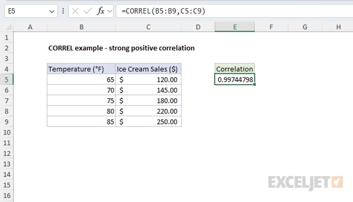
=CORREL(B5:B9,C5:C9) // returns 0.997447985
The result indicates a strong positive correlation between temperature and ice cream sales.
Example #2 - Strong Negative Correlation
Here we examine the relationship between a car’s mileage (miles) and its resale value. As mileage increases, the car’s value decreases proportionally, showing a strong negative correlation.
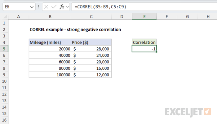
=CORREL(B5:B9,C5:C9) // returns -1
The result confirms a strong negative correlation between car mileage and its market value.
Example #3 - Weak Correlation
This example illustrates two variables with a weak relationship: daily temperature and coffee sales. While there might be some relationship, it’s not very strong.
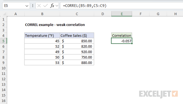
=CORREL(B5:B9,C5:C9) // returns -0.057
The result close to zero indicates a weak negative correlation between temperature and coffee sales.
When to use CORREL
Use CORREL when you need to quantify the linear relationship between two sets of numerical data in Excel. Choose CORREL over COVARIANCE.P or COVARIANCE.S (covariance functions) when you want a standardized measure that’s easy to interpret regardless of the units involved. Use the covariance functions when you care about the magnitude of change in addition to the direction and strength of the relationship between variables.
Key advantages
- Standardized scale (-1 to +1) makes interpretation easier
- Unit-independent - can compare relationships across different measurement scales
- Provides both direction and strength of relationship
- Widely recognized and understood statistical measure
Formula definition
Notes
- Both arrays must contain the same number of values
- Empty cells, text, and logical values are ignored
- Returns #DIV/0! error if either array has zero variance (all values are identical)
- Returns #N/A error if arrays have different lengths
- Only measures linear relationships - may miss non-linear associations
Purpose
Return value
Syntax
=COUNT(value1,[value2],...)
- value1 - An item, cell reference, or range.
- value2 - [optional] An item, cell reference, or range.
Using the COUNT function
The COUNT function returns the count of numeric values in the list of supplied arguments . COUNT takes multiple arguments in the form of value1 , value2 , value3 , etc. Arguments can be individual hardcoded values, cell references, or ranges up to a total of 255 arguments. All numbers are counted, including negative numbers, percentages, dates, times, fractions, and formulas that return numbers. COUNT ignores text values, errors, and empty cells. The COUNT function is similar to the COUNTA function , but COUNTA includes numbers and text in the count.
Examples
The COUNT function counts numeric values and ignores text values:
=COUNT(1,2,3) // returns 3
=COUNT(1,"a","b") // returns 1
=COUNT("apple",100,125,150,"orange") // returns 3
Typically, the COUNT function is used on a range. For example, to count numeric values in the range A1:A10:
=COUNT(A1:A100) // count numbers in A1:A10
In the example shown, COUNT is set up to count numbers in the range B5:B15:
=COUNT(B5:B15) // returns 6
COUNT returns 6, since there are 6 numeric values in the range B5:B15. Text values and blank cells are ignored. Note that dates and times are numbers, and therefore included in the count.
Functions for counting
- To count numbers only, use the COUNT function .
- To count numbers and text, use the COUNTA function .
- To count with one condition, use the COUNTIF function
- To count with multiple conditions, use the COUNTIFS function .
- To count empty cells, use the COUNTBLANK function .
Notes
- COUNT can handle up to 255 arguments.
- COUNT ignores the logical values TRUE and FALSE.
- COUNT ignores text values, errors, and empty cells.
