Explanation
The goal of this example is to count rows in the data where the date joined falls between start and end dates (inclusive) and the age also falls into the age ranges seen in column G. The formula is complicated somewhat by the fact that the age range labels are actually text, so we need to extract a low and high number for each age range as a separate step.
Note: the named ranges shown in this example are entirely optional. They are a way to make the formula easier to enter, read, and copy.
Count between dates
The main function used to solve this problem is COUNTIFS . To explain how this works, we’ll look first at the total seen in cell H6. This total does not take into account age groups, it simply counts all records that fall between the start and end dates. The formula in H6 is:
=COUNTIFS(joined,">="&start,joined,"<="&end)
COUNTIFS is configured with two range/criteria pairs: one to count join dates greater than or equal to the start date in cell H4:
joined,">="&start // greater than or equal to start
and one to count join dates less than or equal to the end date in cell H5:
joined,"<="&end // less than or equal to end
Note that we are concatenating the operators inside the formula with the ampersand (&). The COUNTIFS function belongs to a group of functions that use this syntax.
With this configuration, COUNTIFS returns the total records with a join date greater than or equal to the start and end dates in H4 and H5.
Count between age range
The formula above counts records using the start and end dates, but does not take age range into account. To further restrict the count to the age ranges shown in column G, we need to add two more range/criteria pairs. The first pair restricts the count to ages greater than or equal to the “low” number:
age, ">="&LEFT(G8,FIND("-",G8)-1) // low
Here, we use the FIND and LEFT function to extract the low number. The FIND function returns the position of the hyphen (-) and feeds this number (minus 1) to the LEFT function as the number of characters to extract. LEFT returns zero (“0”), which is concatenated to the greater than or equal to operator (>=). In the end, we have:
age,">=0"
The second range/criteria pair restricts the count to ages less than or equal to the “high” number in the age range:
age,"<="&RIGHT(G8,LEN(G8)-FIND("-",G8)) // high
As before, we use the FIND function to locate the position of the hyphen (-). The result is subtracted from the total of all characters in the cell (calculated with the LEN function ) and this result is given to the RIGHT function for the number of characters to extract from the right side. RIGHT returns 20, which is concatenated to the less than or equal to operator (<=). In the end, we have:
age,"<=20"
As this formula is copied down the range H8:H11, the high and low values in the age ranges are extracted and used as conditions to restrict the count , while the original date logic remains unchanged.
With SUMPRODUCT
This problem can also be solved with the SUMPRODUCT function . To get the total in cell H6, you can use a formula like this:
=SUMPRODUCT((joined>=start)*(joined<=end))
To count by age ranges, the formula in H8, copied down, is:
=SUMPRODUCT((joined>=start)*(joined<=end)*(age>=LEFT(G8,FIND("-",G8)-1)+0)*(age<=RIGHT(G8,LEN(G8)-FIND("-",G8))+0))
Note when checking the age, we need to add zero to the result from the LEFT function and the RIGHT function, because these functions return text, and any text value will cause the age checks to fail. Adding zero is an easy way to convert a number represented as text into a true numeric value. This isn’t necessary with COUNTIFS above, because COUNTIFS does some kind of internal magic to evaluate numeric criteria correctly, even though the criteria is provided as text.
TEXTBEFORE and TEXTAFTER
The new TEXTBEFORE and TEXTAFTER functions can help simplify the formulas above, because they make it easier to parse the age range. The COUNTIFS version can be simplified to:
=COUNTIFS(joined,">="&start,joined,"<="&end,age,">="&TEXTBEFORE(G8,"-"),age,"<="&TEXTAFTER(G8,"-"))
And the SUMPRODUCT version can be written as:
=SUMPRODUCT((joined>=start)*(joined<=end)*(age>=TEXTBEFORE(G8,"-")+0)*(age<=TEXTAFTER(G8,"-")+0))
TEXTBEFORE and TEXTAFTER are currently available in Excel 365 only.
Explanation
In this example, the goal is to count birthdays by year. The source data is an Excel Table named data in the range C5:C16. The birthdays we want to count are in the Birthday column. In column E, the years of interest have been previously entered. The easiest way to solve this problem is with the SUMPRODUCT function, but it can also be solved with COUNTIFS as explained below.
SUMPRODUCT function
The easiest way to solve this problem is to use the SUMPRODUCT function together with the YEAR function like this in cell F5:
=SUMPRODUCT(--(YEAR(data[Birthday])=E5))
Working from the inside out, we use the YEAR function to extract the year from each birthday:
YEAR(data[Birthday]) // extract year
Because there are 12 dates in the list, the YEAR function returns 12 values in an array like this:
{1999;1999;2000;2000;2000;2000;2001;1999;2000;2001;2001;2002}
Next, each value in this array is compared against the year in E5, which is 1999. The result is a new array containing only TRUE and FALSE values:
{TRUE;TRUE;FALSE;FALSE;FALSE;FALSE;FALSE;TRUE;FALSE;FALSE;FALSE;FALSE}
In this array, TRUE represents birth years equal to 1999 and FALSE represents birth years not equal to 1999. We want to count the TRUE values, but because SUMPRODUCT will ignore the logical values TRUE and FALSE, we need to convert these values to 1s and 0s first. To perform this conversion, we use a double negative (–). The result is an array that contains just 1s and 0s, which is returned directly to the SUMPRODUCT function like this:
=SUMPRODUCT({1;1;0;0;0;0;0;1;0;0;0;0})
With only one array to process, SUMPRODUCT sums the array and returns a result of 3 in cell F5. As the formula is copied down, it returns a count of birthdays per year as seen in the worksheet.
Note: The SUMPRODUCT formula above is an example of using Boolean logic in an array operation . This is a powerful and flexible approach to solving many problems in Excel. It is also an important skill with new functions like FILTER and XLOOKUP , which often use this technique to apply multiple criteria ( FILTER example , XLOOKUP example )
COUNTIFS function
The COUNTIFS function can also be used to solve this problem but the formula is more complicated, because COUNTIF only works with ranges , and you can’t extract the years to use as the range argument inside COUNTIFS. Instead, you must create a start and end date for each year. The formula looks like this:
=COUNTIFS(data[Birthday],">="&DATE(E5,1,1),data[Birthday],"<="&DATE(E5,12,31))
In a nutshell, we create a first-of-year date (1-Jan-1999) and an end-of-year date (31-Jan-1999) using the year in E5 with the DATE function :
DATE(E5,1,1) // first day of year
DATE(E5,12,31) // last day of year
The DATE function creates Excel dates with separate year , month , and day arguments. In the example, month and day are hard-coded, and we get year from column E. These dates are concatenated to the greater than or equals to operator (>=) to make criteria1 , and the less than or equals to operator (<=) to make criteria2 . The range for both criteria is data[Birthday] . Notice the operators must be enclosed in double quotes ("").
As the formula is copied down column F, it returns a count of birthdays per year, same as the SUMPRODUCT formula.
Dynamic array solution
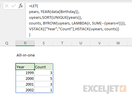
In the latest version of Excel, which supports dynamic array formulas , it is possible to create a single all-in-one formula that builds the entire summary table, including headers, like this:
=LET(
years, YEAR(data[Birthday]),
uyears,SORT(UNIQUE(years)),
counts, BYROW(uyears, LAMBDA(r, SUM(--(years=r)))),
VSTACK({"Year","Count"},HSTACK(uyears, counts))
)
The LET function is used to assign three intermediate variables: years , uyears, and counts . The value for years is created like this:
YEAR(data[Birthday]) // extract years
Here, the YEAR function is used to extract just the year from all dates in data[Birthday] . Because the table contains 12 rows, the result is an array with 12 year values like this:
{1999;1999;2000;2000;2000;2000;2001;1999;2000;2001;2001;2002}
Next, the value for uyears (unique years) is created like this:
SORT(UNIQUE(years)) // get and sort unique years
Out of 12 year values, the UNIQUE function returns just 4 unique years:
{1999;2000;2001;2002} // unique
This array is returned to the SORT function, which returns an array sorted in ascending order:
={1999;2000;2001;2002} // sorted
In this example, it happens that the unique years are already in ascending order, so the SORT function does not change the result from UNIQUE. However, using the SORT function ensures that year values will always appear in order when source data is not sorted.
Next, the BYROW function is used to create a value for counts for each year like this:
BYROW(uyears, LAMBDA(r, SUM(--(years=r)))) // counts
BYROW runs through the uyears values row by row. At each row, it applies this calculation:
LAMBDA(r, SUM(--(years=r)))
The value for r is the year in the “current” row. Inside the SUM function, this value is compared to years . Since years contains all 12 years, the result is an array with 12 TRUE and FALSE results. The TRUE and FALSE values are converted to 1s and 0s with the double negative (–), and the SUM function simply adds up the result, which is the count of birthdays associated with the current row. Since there are 4 unique years, the result from BYROW is an array with 4 counts like this:
={3;5;3;1} // counts
Finally the HSTACK and VSTACK functions are used to assemble a complete table:
VSTACK({"Year","Count"},HSTACK(uyears, counts))
At the top of the table, the array constant {“Year”,“Count”} creates a header row. The HSTACK function combines uyears and counts horizontally, and VSTACK combines the header row and the data to make the final table. The result spills into multiple cells on the worksheet:
Pivot table solution
A Pivot Table is a good solution for this problem as well. This example shows how to count birthdays by month with a Pivot Table.
