Explanation
In this example, the goal is to count test scores in column C that are less than 75. The simplest way to do this is with the COUNTIF function , which takes two arguments , range and criteria :
=COUNTIF(range,criteria)
The test scores in the range C5:C16 and we want to count scores less than 75 , so we configure COUNTIF like this:
=COUNTIF(C5:C16,"<75") // returns 1
Since there is only one score in C5:C16 that is less than 75, COUNTIF returns 1 as a result. Notice that criteria is given as a text value in double quotes (""). This is a requirement of the COUNTIF function which is in a group of eight functions that use a special syntax for criteria . In this syntax, logical operators are joined with numeric values and provided as text.
Less than or equal to
To count cells that are less than or equal to , adjust the formula to use “<=” instead of “<”. In the example shown, the formula in F6 is:
=COUNTIF(C5:C16,"<=75") // returns 2
Here, COUNTIF returns 2 since there are two scores in C5:C16 less than or equal to 75.
Value in another cell
To adjust the formula to use a value in another cell as part of the criteria, you can concatenate the logical operator to the cell reference with the ampersand (&) operator like this:
=COUNTIF(range,"<"&A1)
For example, with 75 in cell A1, the criteria will be “<=75” after concatenation:
=COUNTIF(range,"<="&A1)
=COUNTIF(range,"<=75")
=2
The result will again be 2. If the value in A1 is changed to a different number, COUNTIF will return a new result.
COUNTIFS function
The COUNTIFS function is designed to handle multiple criteria , but can be used just like the COUNTIF function in this example:
=COUNTIFS(C5:C16,"<75") // returns 1
=COUNTIFS(C5:C16,"<=75") // returns 2
Video: How to use the COUNTIFS function
Explanation
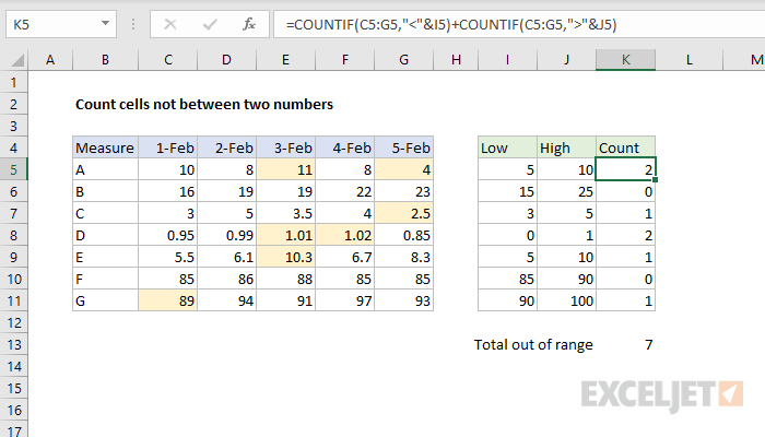
The goal of this example is to count the number of values recorded over 5 days that do not fall between two numbers, a low value, and a high value. In other words, to count values that are “out of range”. Note that each row, labeled A-G, has its own low and high limit, in columns I and J.
You might at first think to use the COUNTIFS function with two criteria. However, because COUNTIFS joins criteria with AND logic, it can’t be used with two criteria in this scenario. The logic of less than low AND greater than high will always fail, and the result will always be zero. Instead, we need OR logic.
One straightforward solution is to use the COUNTIF function twice like this:
=COUNTIF(C5:G5,"<"&I5)+COUNTIF(C5:G5,">"&J5)
The first COUNTIF counts values below the value in I5, and the second COUNTIF counts values above the value in J5. When added together these two results correctly handle the required logic: less than I5 OR greater than J5. Notice the greater than (">") and less than ("<") operators are concatenated to cell references with an ampersand (&) operator , a quirk of RACON functions .
With SUMPRODUCT
A more elegant solution is to use the SUMPRODUCT function with two logical expressions:
=SUMPRODUCT((C5:G5<I5)+(C5:G5>J5))
Notice we don’t need to use concatenation with cell references as with the COUNTIF function above; standard expressions work fine.
This is an example of using boolean algebra with addition (+), which creates OR logic. When these expressions are evaluated, we have two arrays of TRUE and FALSE values like this:
=SUMPRODUCT({FALSE,FALSE,FALSE,FALSE,TRUE}+{FALSE,FALSE,TRUE,FALSE,FALSE})
The math operation automatically coerces the TRUE and FALSE values to 1s and 0s. The result can be visualized like this:
=SUMPRODUCT({0,0,0,0,1}+{0,0,1,0,0})
This results in a single array containing two 1s:
=SUMPRODUCT({0,0,1,0,1})
With only one array to process, SUMPRODUCT sums the items in the array and returns a final result of 2.
Conditional formatting
To easily see which values aren’t between two values, you can use a conditional formatting rule with a formula .

The formula used to highlight the out-of-range values above is:
=OR(C5<$I5,C5>$J5)
More details here .