Explanation
In this example, the goal is to count codes that appear as substrings in a case-sensitive way. The functions COUNTIF and COUNTIFS are both good options for counting text values, but these functions are not case-sensitive, so they can’t be used to solve this problem. The solution is to use the FIND function together with the ISNUMBER function to check for substrings and the SUMPRODUCT function to add up the results.
The FIND function is always case-sensitive and takes three arguments: find_text, within_text , and start_num . Find_text is the text we want to look for, and within_text is the text we are looking inside of. Start_num is the position at which to start looking in find_text . Start_num defaults to 1, so we aren’t providing a value in this case, because we always want FIND to start at the first character. When find_text is found inside within_text , FIND returns the position of the found text as a number:
=FIND("ABC","ABC-101") // returns 1
=FIND("ABC","10-ABC-101") // returns 4
When find_text is not found , FIND returns the #VALUE! error:
=FIND("ABC","XYZ-101") // returns #VALUE!
This means we can use the ISNUMBER function to convert the result from FIND into a TRUE and FALSE value. Any number will result in TRUE, and any error will result in FALSE:
=ISNUMBER(FIND("ABC","ABC-101")) // returns TRUE
=ISNUMBER(FIND("XYZ","ABC-101")) // returns FALSE
This idea is explained in more detail here .
In the example shown, we have four substrings in column D and a variety of codes in B5:B15, which is the named range data . We want to count how many times each substring in D5:D8 appears in B5:B15, and this count needs to be case-sensitive.
The formula in E5, copied down, is:
=SUMPRODUCT(--ISNUMBER(FIND(D5,data)))
Working from the inside-out, the FIND function is used to look for a substring like this:
FIND(D5,data)
FIND checks for the value in D5 (“ABC”) in all cells in the data . Because we give FIND multiple values in the within_text argument, it returns multiple results. In total, FIND returns 11 values (one for each code in B5:B15) in an array like this:
{4;#VALUE!;#VALUE!;#VALUE!;#VALUE!;#VALUE!;#VALUE!;4;4;#VALUE!;4}
Each number represents a cell in B5:B15 that contains “ABC”. Each #VALUE! represents a value in B5:B15 that does not contain “ABC”. Looking more closely, we can see that FIND found “ABC” in 4 cells out of 11. This array is returned directly to the ISNUMBER function which converts each value to TRUE or FALSE:
ISNUMBER({4;#VALUE!;#VALUE!;#VALUE!;#VALUE!;#VALUE!;#VALUE!;4;4;#VALUE!;4})
ISNUMBER returns an array of 11 TRUE and FALSE values:
{TRUE;FALSE;FALSE;FALSE;FALSE;FALSE;FALSE;TRUE;TRUE;FALSE;TRUE}
Because we want to count results, we use a double-negative (–) to convert TRUE and FALSE values into 1’s and 0’s:
--{TRUE;FALSE;FALSE;FALSE;FALSE;FALSE;FALSE;TRUE;TRUE;FALSE;TRUE}
The resulting array looks like this:
{1;0;0;0;0;0;0;1;1;0;1} // 11 results
Using the double-negative like this is an example of Boolean logic , a technique for handling TRUE and FALSE values like 1’s and 0’s. The resulting array is delivered directly to the SUMPRODUCT function:
=SUMPRODUCT({1;0;0;0;0;0;0;1;1;0;1}) // returns 4
With just one array to process, SUMPRODUCT sums all numbers in the array and returns the final result: 4. As the formula is copied down, it returns a count of each substring in column D. The reference to data does not change, because a named range automatically behaves like an absolute reference .
Note: Because SUMPRODUCT can handle arrays natively, it’s not necessary to use Control+Shift+Enter to enter this formula.
Explanation
In this example, the goal is to count cells in the range B5:B15 that contain either “x” or “y”, where x and y are both text strings . When you count cells with “OR logic”, you need to be careful not to double count. For example, if you are counting cells that contain “blue” or “green”, you can’t just add together two COUNTIF functions, because you may double count cells that contain both “blue” and “green”. The article below explains two options, a single formula based on the SUMPRODUCT function, and a second option based on the COUNTIF function and a helper column. For convenience, the range B5:B15 is named data .
Note: The main formula described on this page is case-sensitive because the FIND function is case-sensitive. If you want a formula that is not case-sensitive, you can substitute the SEARCH function for the FIND function.
SUMPRODUCT formula
One way to solve this problem is to use the SUMPRODUCT function with ISNUMBER + FIND . The formula in E5 is:
=SUMPRODUCT(--((ISNUMBER(FIND("blue",data))+ISNUMBER(FIND("green",data)))>0))
This formula is based on a formula explained here that finds text in a cell. The main work is done with the FIND function and the ISNUMBER function , like this:
ISNUMBER(FIND("red","A red hat") // returns TRUE
FIND returns the number 4 since “red” starts at character 4, and ISNUMBER returns TRUE because 4 is a number. If the text is not found, FIND returns a #VALUE! error and ISNUMBER returns FALSE:
ISNUMBER(FIND("blue","A red hat") // returns FALSE
When given a range of cells, this snippet will return an array of TRUE/FALSE values, one value for each cell in the range. Going back to the formula in the example, and working from the inside out, we look for “blue” like this:
ISNUMBER(FIND("blue",data)
Since the named range data (B5:B15) contains 11 values, we get back an array with 11 TRUE/FALSE values like this:
{TRUE;TRUE;FALSE;TRUE;FALSE;TRUE;FALSE;FALSE;FALSE;TRUE;TRUE}
Each TRUE corresponds to a cell in data that contains “blue”. We look for “green” in the same way:
ISNUMBER(FIND("green",data)
And this snippet also returns an array with 11 results:
{TRUE;FALSE;TRUE;TRUE;FALSE;TRUE;FALSE;FALSE;FALSE;TRUE;TRUE}
Next, we add these arrays together with the addition operator (+). The math operation changes the TRUE and FALSE values to 1s and 0s, and the result is a single array:
{2;1;1;2;0;2;0;0;0;2;2}
In this array, a 1 indicates a cell that contains either “blue” or “green” and a 2 indicates a cell that contains both “blue” and “green”. Next, we need to add these numbers up, but we don’t want to double count. To make sure that any value greater than zero is just counted once, we first force all values to TRUE or FALSE with “>0”:
{2;1;1;2;0;2;0;0;0;2;2})>0
This again creates an array of TRUE and FALSE values:
{TRUE;TRUE;TRUE;TRUE;FALSE;TRUE;FALSE;FALSE;FALSE;TRUE;TRUE}
Because we want numbers, we use a double-negative (–) to change the TRUE and FALSE values to 1s and 0s to yield an array like this:
{1;1;1;1;0;1;0;0;0;1;1}
In this array, a 1 indicates a cell in data that contains “blue” or “green” and a 0 indicates a cell that does not contain “blue” or “green”. To summarize the operations above:
=SUMPRODUCT(--(({2;1;1;2;0;2;0;0;0;2;2})>0))
=SUMPRODUCT({1;1;1;1;0;1;0;0;0;1;1})
Finally, SUMPRODUCT returns the sum of all values in the array, 7, as a final result.
Note: this formula is an example of using Boolean algebra to apply “OR logic” in a formula.
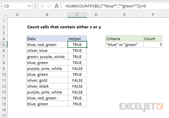
Helper column solution
Another way to solve this problem is with a helper column . This breaks up a more complex problem into parts. To check each cell in B5:B15 for “blue” or “green”, we can use the COUNTIF function with an array constant like this:
=SUM(COUNTIF(B5,{"*blue*","*green*"}))>0
Because we give COUNTIF an array that contains two items for criteria, it returns an array that contains two counts: one for “blue” and one for “green”. The asterisk (*) is a wildcard we can use for a contains search. To prevent double counting, we add the counts up with the SUM function and then force the result to TRUE/FALSE with “>0”. As the formula is copied down, we get a TRUE or FALSE value in column C for each value in column B.
This is how the helper column looks on the worksheet:
To sum up all TRUE in C5:C15, we can use the SUMPRODUCT function. The formula in F5 is:
=SUMPRODUCT(--C5:C15)
The double negative (–) coerces the TRUE and FALSE values to 1s and 0s:
=SUMPRODUCT({1;1;1;1;0;1;0;0;0;1;1}) // returns 7
and SUMPRODUCT returns 7 as a final result.
