Explanation
In this example, the goal is to count cells in the range B5:B15 that contain either “x” or “y”, where x and y are both text strings . When you count cells with “OR logic”, you need to be careful not to double count. For example, if you are counting cells that contain “blue” or “green”, you can’t just add together two COUNTIF functions, because you may double count cells that contain both “blue” and “green”. The article below explains two options, a single formula based on the SUMPRODUCT function, and a second option based on the COUNTIF function and a helper column. For convenience, the range B5:B15 is named data .
Note: The main formula described on this page is case-sensitive because the FIND function is case-sensitive. If you want a formula that is not case-sensitive, you can substitute the SEARCH function for the FIND function.
SUMPRODUCT formula
One way to solve this problem is to use the SUMPRODUCT function with ISNUMBER + FIND . The formula in E5 is:
=SUMPRODUCT(--((ISNUMBER(FIND("blue",data))+ISNUMBER(FIND("green",data)))>0))
This formula is based on a formula explained here that finds text in a cell. The main work is done with the FIND function and the ISNUMBER function , like this:
ISNUMBER(FIND("red","A red hat") // returns TRUE
FIND returns the number 4 since “red” starts at character 4, and ISNUMBER returns TRUE because 4 is a number. If the text is not found, FIND returns a #VALUE! error and ISNUMBER returns FALSE:
ISNUMBER(FIND("blue","A red hat") // returns FALSE
When given a range of cells, this snippet will return an array of TRUE/FALSE values, one value for each cell in the range. Going back to the formula in the example, and working from the inside out, we look for “blue” like this:
ISNUMBER(FIND("blue",data)
Since the named range data (B5:B15) contains 11 values, we get back an array with 11 TRUE/FALSE values like this:
{TRUE;TRUE;FALSE;TRUE;FALSE;TRUE;FALSE;FALSE;FALSE;TRUE;TRUE}
Each TRUE corresponds to a cell in data that contains “blue”. We look for “green” in the same way:
ISNUMBER(FIND("green",data)
And this snippet also returns an array with 11 results:
{TRUE;FALSE;TRUE;TRUE;FALSE;TRUE;FALSE;FALSE;FALSE;TRUE;TRUE}
Next, we add these arrays together with the addition operator (+). The math operation changes the TRUE and FALSE values to 1s and 0s, and the result is a single array:
{2;1;1;2;0;2;0;0;0;2;2}
In this array, a 1 indicates a cell that contains either “blue” or “green” and a 2 indicates a cell that contains both “blue” and “green”. Next, we need to add these numbers up, but we don’t want to double count. To make sure that any value greater than zero is just counted once, we first force all values to TRUE or FALSE with “>0”:
{2;1;1;2;0;2;0;0;0;2;2})>0
This again creates an array of TRUE and FALSE values:
{TRUE;TRUE;TRUE;TRUE;FALSE;TRUE;FALSE;FALSE;FALSE;TRUE;TRUE}
Because we want numbers, we use a double-negative (–) to change the TRUE and FALSE values to 1s and 0s to yield an array like this:
{1;1;1;1;0;1;0;0;0;1;1}
In this array, a 1 indicates a cell in data that contains “blue” or “green” and a 0 indicates a cell that does not contain “blue” or “green”. To summarize the operations above:
=SUMPRODUCT(--(({2;1;1;2;0;2;0;0;0;2;2})>0))
=SUMPRODUCT({1;1;1;1;0;1;0;0;0;1;1})
Finally, SUMPRODUCT returns the sum of all values in the array, 7, as a final result.
Note: this formula is an example of using Boolean algebra to apply “OR logic” in a formula.
Helper column solution
Another way to solve this problem is with a helper column . This breaks up a more complex problem into parts. To check each cell in B5:B15 for “blue” or “green”, we can use the COUNTIF function with an array constant like this:
=SUM(COUNTIF(B5,{"*blue*","*green*"}))>0
Because we give COUNTIF an array that contains two items for criteria, it returns an array that contains two counts: one for “blue” and one for “green”. The asterisk (*) is a wildcard we can use for a contains search. To prevent double counting, we add the counts up with the SUM function and then force the result to TRUE/FALSE with “>0”. As the formula is copied down, we get a TRUE or FALSE value in column C for each value in column B.
This is how the helper column looks on the worksheet:
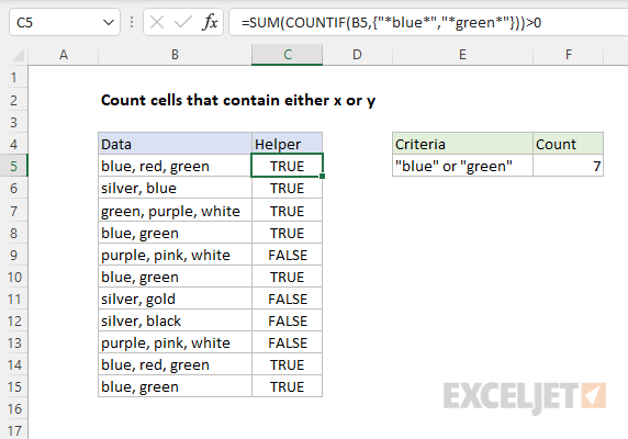
To sum up all TRUE in C5:C15, we can use the SUMPRODUCT function. The formula in F5 is:
=SUMPRODUCT(--C5:C15)
The double negative (–) coerces the TRUE and FALSE values to 1s and 0s:
=SUMPRODUCT({1;1;1;1;0;1;0;0;0;1;1}) // returns 7
and SUMPRODUCT returns 7 as a final result.
Explanation
In this example, the goal is to count errors in the range B5:B15, which is named data for convenience. The article below explains several different approaches, depending on your needs. For background, this article: Excel Formula Errors .
COUNTIF function
One way to count individual errors is with the COUNTIF function like this:
=COUNTIF(data,"#N/A") // returns 1
=COUNTIF(data,"#VALUE!") // returns 1
=COUNTIF(data,"#DIV/0!") // returns 0
This is an odd syntax since technically errors are not text values . But COUNTIF is in a group of eight functions that have some quirks , and this is one of them. During calculation, COUNTIF is able to resolve the text into the given error and return a count of that error. One limitation of this approach is that there is no simple way to count all error types with a single formula. You might think we can use COUNTIF like this:
=COUNTIF(ISERROR(data),TRUE) // fails
The idea here is that the ISERROR function will return TRUE or FALSE, and COUNTIF will count the TRUE results. However, if you try to enter this formula, Excel won’t let you. This is a case where COUNTIF won’t work because it won’t allow an " array operation " in place of a normal range. One solution is to use SUMPRODUCT with ISERROR, as explained below.
SUMPRODUCT function
A better way to count errors in a range is to use the SUMPRODUCT function with the ISERROR function and Boolean logic . The SUMPRODUCT function accepts one or more arrays, multiplies the arrays together, and returns the “sum of products” as a final result. If only one array is supplied, SUMPRODUCT simply returns the sum of items in the array. In the example shown, the formula in E6 is:
=SUMPRODUCT(--ISERROR(data))
Working from the inside out, the ISERROR function returns TRUE when a cell contains an error, and FALSE if not. Because there are eleven cells in the range B5:B15, ISERROR evaluates each cell and returns 11 results in an array like this:
{FALSE;FALSE;FALSE;TRUE;FALSE;FALSE;FALSE;TRUE;FALSE;FALSE;FALSE}
Next, we use a double negative (–) to convert the TRUE and FALSE values to 1s and 0s. The resulting array inside the SUMPRODUCT function looks like this:
=SUMPRODUCT({0;0;0;1;0;0;0;1;0;0;0})
Finally, SUMPRODUCT sums the items in this array and returns the total, which is 2 in this case.
ISERR option
=SUMPRODUCT(--ISERR(data)) // returns 1
Since one of the errors shown in the example is #N/A, this formula returns 1 instead of 2.
Count by error code
Each Excel formula error is associated with a numeric error code ( complete list here ). You can retrieve this code with the ERROR.TYPE function . To count errors by numeric code, you can use ERROR.TYPE instead of ISERROR. For example to count #VALUE! errors, which have a numeric code of 3, you can use a formula like this:
=SUMPRODUCT(--(IFERROR(ERROR.TYPE(data),0)=3))
In an ironic twist, we need the IFERROR function to help us here. The ERROR.TYPE function will return a numeric code for any formula error. However, if a cell does not contain an error, ERROR.TYPE itself returns an #N/A error, which will bubble to the top and cause the entire formula to return #N/A. We use IFERROR to map the #N/A errors to zero so that we can compare the results from ERROR.TYPE to 3 without trouble. This part of the formula evaluates like this:
=IFERROR(ERROR.TYPE(data),0)=3)
=IFERROR({#N/A;#N/A;#N/A;3;#N/A;#N/A;#N/A;7;#N/A;#N/A;#N/A},0)=3)
={0;0;0;3;0;0;0;7;0;0;0}=3
={FALSE;FALSE;FALSE;TRUE;FALSE;FALSE;FALSE;FALSE;FALSE;FALSE;FALSE}
Notice in the second step above, we see error code 3 and error code 7. This indicates the #VALUE! and #N/A error in data (B5:B15). After IFERROR runs, the #N/A errors are gone and replaced with zeros, as you can see in the third step. This lets us check for error code 3 without trouble. From there, we use a double negative to convert the TRUE and FALSE values to 1s and 0s and the resulting array is returned directly to SUMPRODUCT:
=SUMPRODUCT({0;0;0;1;0;0;0;0;0;0;0}) // returns 1
The final result is 1, since there is one error in data with an error code of 3.
Note: In Excel 365 and Excel 2021 you can use the SUM function instead of SUMPRODUCT in all formulas above if you prefer, with some caveats. This article provides a complete explanation .
