Explanation
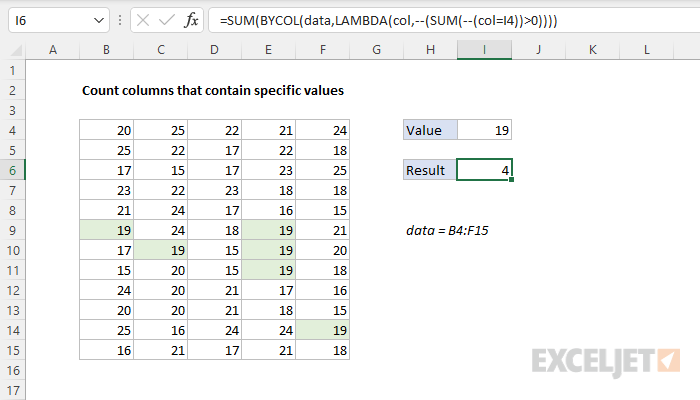
In this example, the goal is to count the number of columns in the data that contain 19 (the value in cell I4). The main challenge in this problem is that the value might appear in any row, and more than once in the same column. If we wanted to simply count the total number of times a value appeared in a range, we could use the COUNTIF function . But we need a more advanced formula to count columns that may contain multiple instances of a specific value. The explanation below discusses two options: one based on the MMULT function , and one based on the newer BYCOL function .
MMULT option
One option for solving this problem is the MMULT function . The MMULT function returns the matrix product of two arrays, sometimes called the “dot product”. The result from MMULT is an array that contains the same number of rows as array1 and the same number of columns as array2 . The MMULT function takes two arguments , array1 and array2 , both of which are required. The column count in array1 must equal the row count in array2 . In the example shown, the formula in I6 is:
=SUM(--(MMULT(TRANSPOSE(ROW(data)^0),--(data=I4))>0))
Working from the inside out, the logical criteria used in this formula is:
--(data=I4)
where data is the named range B4:F15. This expression generates a TRUE or FALSE result for every value in data, and the double negative (–) coerces the TRUE and FALSE values to 1s and 0s, respectively. The result is an array of 1s and 0s like this:
{0,0,0,0,0;0,0,0,0,0;0,0,0,0,0;0,0,0,0,0;0,0,0,0,0;1,0,0,1,0;0,1,0,1,0;0,0,0,1,0;0,0,0,0,0;0,0,0,0,0;0,0,0,0,1;0,0,0,0,0}
Like the original data, this array is 12 rows by 5 columns (12 x 5) and is delivered directly to the MMULT function as array2 . Array1 is derived with this snippet:
TRANSPOSE(ROW(data)^0)
This is the tricky part of the formula. The ROW function is used to generate a numeric array of the right size. To perform matrix multiplication with MMULT, the column count in array1 (12) must equal the row count in array2 (12). ROW returns a 12-row array, which is raised to the power of zero, and converted with the TRANSPOSE function into a 12-column array:
=TRANSPOSE(ROW(data)^0)
=TRANSPOSE({4;5;6;7;8;9;10;11;12;13;14;15}^0)
=TRANSPOSE({1;1;1;1;1;1;1;1;1;1;1;1})
={1,1,1,1,1,1,1,1,1,1,1,1}
With both arrays in place, the MMULT function runs and returns an array with 1 row and 5 columns, {1,1,0,3,1}. This is the data we can use to solve the problem. Each non-zero number represents a column that contains the number 19. We can now simplify the formula to:
=SUM(--({1,1,0,3,1}>0))
We check for non-zero entries with >0 and again coerce TRUE FALSE to 1 and 0 with a double negative (–) to get a final array inside SUM:
=SUM({1,1,0,1,1})
In this array, 1 represents a column that contains 19 and 0 represents a column that does not contain 19. The SUM function returns a final result of 4, the count of all columns that contain the number 19.
BYCOL option
The BYCOL function applies a LAMBDA function to each column in a given array and returns one result per column in a single array . The purpose of BYCOL is to process data in an array or range in a “by column” fashion. For example, if BYCOL is given an array with 5 columns, BYCOL will return an array with 5 results. In this example, we can use BYCOL like this:
=SUM(BYCOL(data,LAMBDA(col,--(SUM(--(col=I4))>0))))
The BYCOL function iterates through the named range data (B4:D15) one column at a time. At each column, BYCOL evaluates and stores the result of the supplied LAMBDA function:
LAMBDA(col,--(SUM(--(col=I4))>0))
Working from the inside out, the logic here checks for values in col that are equal to I4, which results in an array of TRUE and FALSE values. The TRUE and FALSE values are coerced to 1s and 0s with the double negative (–), and the SUM function sums the result. Next, we check if the result from SUM is > 0 and coerce that result to a 1 or 0 with another double negative. After BYCOL runs, we have an array with one result per column, either a 1 or 0:
{1,1,0,1,1} // result from BYCOL
The formula can now be simplified as follows:
=SUM({1,1,0,1,1}) // returns 4
In the last step, the SUM function sums the items in the array and returns a final result of 4.
Literal contains
If you need to check for specific text values, in other words, literally check to see if cells contain certain text values, you can change the logic in the formula on this page to use the ISNUMBER and SEARCH function. For example, to count cells/rows that contain “apple” you can use:
=ISNUMBER(SEARCH("apple",data))
Details on how this formula works here .
Explanation
You might wonder why we aren’t using COUNTIF or COUNTIFS . These functions seem like the obvious solution. However, without adding a helper column that contains a weekday value, there is no way to create criteria for COUNTIF to count weekdays in a range of dates. Instead, we use the versatile SUMPRODUCT function , which handles arrays gracefully without the need to use Control + Shift + Enter. We are using SUMPRODUCT with just one argument, which consists of this expression:
--(WEEKDAY(dates,2)=E5)
Working from the inside out, the WEEKDAY function is configured with the optional argument 2, which causes it to return numbers 1-7 for the days Monday-Sunday, respectively. This makes it easier to list the days in order with the numbers in column E in sequence. WEEKDAY evaluates each date in dates (B5:B15) and returns a number. Because we are giving WEEKDAY 11 dates, we get back an array that contains 11 results like this:
{6;1;1;6;3;7;5;6;5;3;2}
Each number in this array corresponds to a day of the week, with Mondays equal to 1 and Sundays equal to 7. Next, the numbers returned by WEEKDAY are compared to the value in E5, which is 1:
{6;1;1;6;3;7;5;6;5;3;2}=1
The result is an array of TRUE/FALSE values like this:
{FALSE;TRUE;TRUE;FALSE;FALSE;FALSE;FALSE;FALSE;FALSE;FALSE;FALSE}
In this array, TRUE corresponds to dates that fall on Monday and FALSE represents other days of the week. SUMPRODUCT only works with numbers (not text or Booleans) so we use a double-negative (–) to coerce the TRUE/FALSE values to 1s and 0s. The result is delivered directly to the SUMPRODUCT function:
=SUMPRODUCT({0;1;1;0;0;0;0;0;0;0;0}) // returns 2
With just one array to process, SUMPRODUCT sums the items and returns 2 as a final result, since there are two Mondays in the dates.
Dealing with blank dates
If you have blank cells in the list of dates, you will get incorrect results, since the WEEKDAY function will return a result even when there is no date. To handle empty cells, you can adjust the formula as follows:
=SUMPRODUCT((WEEKDAY(dates,2)=E5)*(dates<>""))
Multiplying by the expression (dates<>"") is one way to “cancel out” empty cells.
Without day numbers
The day numbers in column E make the formula easier to understand and write. However, since the day names are already in the range D5:D11, which is named days , it is possible to write a formula that doesn’t use column E at all by using the MATCH function like this:
=SUMPRODUCT(--(WEEKDAY(dates,2)=MATCH(D5,days,0)))
This works because the MATCH function simply returns the position of each day name in days :
MATCH(D5,days,0) // returns 1
MATCH(D6,days,0) // returns 2
MATCH(D7,days,0) // returns 3
Otherwise, the formula works the same way and returns the same counts as the original formula.
