Explanation
In this example, the goal is to count numbers that contain leading zeros. In cell E5, we have the code “009875” and we want to count how many times this code appears in the range B5:B16. The challenge is that Excel can be finicky with leading zeros. Technically, the values in B5:B16 are text , as is the value in E5. However, sometimes text values that contain numbers are converted to numeric values as they go through Excel’s calculation engine. When this happens, the leading zeros will be silently removed, which can cause an incorrect result. The article below explains the problem in more detail. For convenience, code (B5:B16) and qty (C5:C16) are named ranges .
COUNTIF with leading zeros
A common situation where leading zeros do not behave as expected is when functions like COUNTIF , COUNTIFS , SUMIF , SUMIFS , etc. are configured to use numbers with leading zeros. To demonstrate this problem, consider the formula below:

Here the COUNTIF function is set up to count values in B4:B8 that are equal to “01”. We expect a result of 1, but COUNTIF returns 5.
=COUNTIF(B4:B8,"01") // returns 5
Somewhere in the calculation process, the leading zeros get dropped and all cells evaluate to 1. This is clearly not the result we want, and shows a limitation of the COUNTIF function. Similarly, if we apply COUNTIF to the worksheet shown above, we get the incorrect result of 4:
=COUNTIF(code,E5) // returns 4
The leading zeros in “009875” are stripped, and 9875 is counted 4 times, when the correct result for “009875"is 2.
Note: COUNTIF is in a group of 8 functions that share some particular quirks and limitations.
SUMPRODUCT solution
A simple solution to this problem is to use the SUMPRODUCT function like this:
=SUMPRODUCT(--(code=E5))
Working from the inside out, we are using the following expression as a logical test :
code=E5
Because code is the named range B5:B16, which contains 12 values, the expression yields 12 TRUE/FALSE results in an array like this:
{FALSE;FALSE;FALSE;TRUE;FALSE;FALSE;FALSE;FALSE;TRUE;FALSE;FALSE;FALSE}
The TRUE values in the array correspond to the cells in B5:B16 that contain “009875”. You can see we have TRUE at the fourth cell (B8) and the ninth cell (B13).
Next, we use a double negative (–) to coerce the TRUE/FALSE values to 1s and 0s, which creates the following array:
{0;0;0;1;0;0;0;0;1;0;0;0}
This array is delivered directly to the SUMPRODUCT function, which sums the array and returns a final result:
=SUMPRODUCT({0;0;0;1;0;0;0;0;1;0;0;0}) // returns 2
This is an example of using Boolean algebra in Excel , and you will see many more advanced formulas use this technique. The nice thing about this approach is that it can be easily extended, as explained below.
Sum quantities
As you might have guessed, if you try to use the SUMIF function to sum the quantities associated with code “009875”, the same problem will occur. The formula below returns 14, when the correct result is 7:
=SUMIF(code,E5,qty) // returns 14
The cause of the problem is the same: the leading zeros in “009875” get stripped during the SUMIF calculation, which causes “009875” to be grouped together with “9875”, and SUMIF sums the quantities associated with both codes.
One of the nicest things about using SUMPRODUCT to perform conditional counts as we did above, is that we can easily extend the logic to perform conditional sums. In this case, all we need to do is multiply the counting logic by the named range qty (C5:C16) like this:
=SUMPRODUCT(--(code=E5)*qty)
This is the formula used in cell G5 of the worksheet. Since we already know that the expression:
--(code=E5)
results in an array of 1s and 0s, we can simplify the formula like this:
=SUMPRODUCT({0;0;0;1;0;0;0;0;1;0;0;0}*qty)
Then, evaluating quantities ( qty ), we get:
=SUMPRODUCT({0;0;0;1;0;0;0;0;1;0;0;0}*{3;6;4;2;5;6;2;4;5;1;3;3})
After the two arrays are multiplied together we have:
=SUMPRODUCT({0;0;0;2;0;0;0;0;5;0;0;0}) // returns 7
Notice how the zeros in the first array “cancel out” the irrelevant quantities in the second array. In other words, the exact same logic we used to count code “009875” is used to sum quantities associated with code “009875”. The final result from SUMPRODUCT is 7.
SUMPRODUCT is a workhorse function that can solve many tricky problems in Excel. See more examples here .
Note: technically the double negative (–) is not needed in the formula to sum quantities above because the math operation of multiplying the two arrays together will automatically coerce the TRUE and FALSE values in the first arrays with 1s and 0s. However, the double negative does no harm and makes the counting and summing formulas easier to compare.
Explanation
In this example, the goal is to count the value in cell B5 (“Steven”) in the sheets listed in B11:B13. The workbook shown in the example has four worksheets in total. The first sheet is named “Master” and contains the search string, the range, and the sheets to include in the count, as seen in the screenshot above. The next three sheets, “Sheet1”, “Sheet2”, and “Sheet3” each contain 1000 random first names in the range B4:F203. The table in each sheet looks like this:
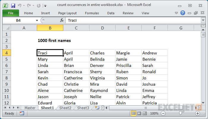
Note that the range (B4:F203) must be adjusted to suit your data.
COUNTIF function
The COUNTIF function returns the count of cells that meet one or more criteria and supports logical operators (>,<,<>,=) and wildcards (*,?) for partial matching. One way to solve this problem is to use the COUNTIF function three times in a formula like this:
=COUNTIF(Sheet1!B4:F203,B5)+COUNTIF(Sheet2!B4:F203,B5)+COUNTIF(Sheet3!B4:F203,B5)
With “Steven” in cell B5, this formula returns 16. This formula works but becomes cumbersome as the number of sheets increases. You might think you could use a 3D reference like this:
=COUNTIF(Sheet1:Sheet3!B4:F203,B5)
However, COUNTIF is in a group of eight functions that have some particular quirks . One of these quirks is that you can’t use a 3D reference for the range argument. As a workaround, you can use the INDIRECT function to assemble an array constant, then feed that into COUNTIF. This approach helps streamline the formula as explained below.
COUNTIF with INDIRECT
The INDIRECT function converts a given text string into a proper Excel reference:
=INDIRECT("A1") // returns A1
We can use INDIRECT in this example to create an array constant that contains all three range references as text. In the example shown, the formula in cell D5 is:
=SUMPRODUCT(COUNTIF(INDIRECT("'"&sheets&"'!"&B8),B5))
Working from the inside out, the INDIRECT function is used to assemble a reference to all three ranges like this:
INDIRECT("'"&sheets&"'!"&B8)
Because the named range sheets contains three cells, the code expands like this:
INDIRECT({"'Sheet1'!B4:F203";"'Sheet2'!B4:F203";"'Sheet3'!B4:F203"})
The result in INDIRECT is an array constant that contains three text strings, each representing a range on each of the three sheets. INDIRECT will evaluate the text values and pass the references into COUNTIF as the range argument. For reasons that are somewhat mysterious, COUNTIF will accept the result from INDIRECT without complaint. Because COUNTIF receives more than one range, it will return more than one result in an array like this:
COUNTIF(INDIRECT("'"&sheets&"'!"&B8) // returns {5;6;5}
The code above will return three counts in an array to the SUMPRODUCT function:
=SUMPRODUCT({5;6;5})
With just one array to process, SUMPRODUCT sums the items in the array and returns 16 as a final result. Note that INDIRECT is a volatile function and can impact workbook performance.
VSTACK function
In the current version of Excel, you can use the VSTACK function with a 3D reference to achieve the same result with a more elegant formula:
=SUMPRODUCT(--(VSTACK(Sheet1:Sheet3!B4:F203)=B5))
The VSTACK function combines the three ranges vertically into a single range and feeds the result into the SUMPRODUCT function . Each cell in the combined range is compared to the value in cell B5 (“Steven”) resulting in a large array containing only TRUE and FALSE values. We then use a double negative (–) to convert the TRUE and FALSE values into their numeric equivalents, 1 and 0. The numeric array is returned to SUMPRODUCT, which sums all items in the array and returns 16 as a final result. This is an example of using Boolean logic , a common way to solve more complicated problems in Excel.
Note: In Excel 365 and Excel 2021 you can use the SUM function instead of SUMPRODUCT if you prefer in both formulas above. This article provides more detail .
