Explanation
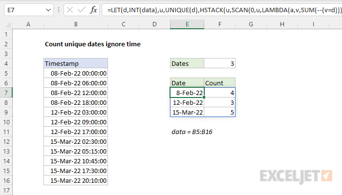
In this example, the goal is to count the unique dates in a range of timestamps (i.e. dates that contain dates and times). In addition, we also want to create the table of results seen in E7:F9. For convenience, data is the named range B5:B16.
Basic count
To get a count of individual dates that occur in B5:B16, ignoring time values, the formula in F4 is:
=COUNT(UNIQUE(INT(data)))
Working from the inside out, the INT function is used to remove the time values from the timestamps like this:
INT(data) // remove time
This works because Excel dates are just serial numbers and Excel times are fractional dates that appear as decimal values. The INT function simply removes the decimal portion of the date, leaving the serial number intact. Because we are giving the INT function 12 separate values, INT returns 12 results in an array like this:
{44600;44600;44600;44600;44604;44604;44604;44635;44635;44635;44635;44635}
Each serial number in this array represents a date in data . Next, the UNIQUE function is used to remove duplicate dates. The two functions work together like this:
UNIQUE(INT(data)) // returns {44600;44604;44635}
Because there are 3 unique dates, UNIQUE returns 3 serial numbers in an array like this:
{44600;44604;44635}
This array is delivered directly to the COUNT function:
=COUNT({44600;44604;44635}) // returns 3
and the COUNT function (which counts numbers only) returns 3 as a final result.
Summary table in two parts
An easy way to create the summary table seen in the worksheet is to use two formulas. To list the 3 unique dates starting in cell D7, you can use:
=UNIQUE(INT(data)) // unique dates
To count how many times each date occurs in the data, you can enter this formula in cell F7 and copy it down:
=SUM(--(INT(data)=K7))
Note: we can’t use the COUNTIF function in this case (which would be easier) because we don’t have the dates without times in an actual range . Instead, the dates exist in an array returned by the INT function. COUNTIF requires a range for the range argument.
All-in-one summary table
To create an all-in-one summary table that lists the unique dates along with a count for each date, you can use an advanced formula like this:
=LET(d,INT(data),u,UNIQUE(d),HSTACK(u,SCAN(0,u,LAMBDA(a,v,SUM(--(v=d))))))
The LET function is used to assign intermediate results to named variables. First, we use INT to strip times from dates and assign the result to d . Then we feed d into UNIQUE (to get unique dates) and assign the result to u. Next, we use the HSTACK function to combine two arrays. Array1 is u (the unique dates), and array2 is generated with the SCAN function :
SCAN(0,u,LAMBDA(a,v,SUM(--(v=d))))
With an initial value of zero, SCAN iterates through each date in u and runs a custom LAMBDA function to count how many times the date appears in d :
LAMBDA(a,v,SUM(--(v=d))
The count is generated with boolean logic and the SUM function . The result from SCAN is an array with 3 counts:
{4;3;5}
This array is returned to HSTACK as array2 . HSTACK joins array1 and array2 together horizontally, and returns the 2-column array as a final result.
Explanation
This example uses the UNIQUE function to extract unique values. When UNIQUE is provided with the range B5:B16, which contains 12 values, it returns the 7 unique values seen in D5:D11. These are returned directly to the COUNTA function as an array like this:
=COUNTA({"red";"amber";"green";"blue";"purple";"pink";"gray"})
Unlike the COUNT function , which counts only numbers, COUNTA counts both text and numbers. Since there are seven items in array , COUNTA returns 7. This formula is dynamic and will recalculate immediately when source data is changed.
With a cell reference
You can also refer to a list of unique values already extracted to the worksheet with the UNIQUE function using a special kind of cell reference. The formula in D5 is:
=UNIQUE(B5:B16)
Which returns the seven values seen in D5:D11. To count these values with a dynamic reference, you can use a formula like this:
=COUNTA(D5#)
The hash character (#) tells Excel to refer to the spill range created by UNIQUE. Like the all-in-one formula above, this formula is dynamic and will adapt when data is added or removed from the original range.
Count unique and ignore blank cells
If blank (i.e., empty) cells exist in the range, the can increase the count by 1. The problem is that the empty cells evaluate to zero (0), and UNIQUE returns the zero along with other unique values. Then COUNTA counts the zero. To count unique values while ignoring blank cells, you can add the FILTER function like this:
=COUNTA(UNIQUE(FILTER(data,data<>"")))
Here, FILTER is configured to select only non-empty cells, so empty cells are excluded and never make it to the UNIQUE function. This approach is explained in more detail here . You can also filter unique values with criteria .
No data
One limitation of the formula above is that it will incorrectly return 1 even if there aren’t any values in the data range. This alternative formula will count all values returned by UNIQUE that have a length greater than zero. In other words, it will count all values with at least one character:
=SUM(--(LEN(UNIQUE(B5:B16))>0))
Here, the LEN function is used to check the length of results from UNIQUE. The lengths are then checked to see if they are greater than zero, and results are counted with the SUM function. This is an example of boolean logic . This formula will also exclude empty cells from results.
Dynamic source range
UNIQUE won’t automatically change the source range if data is added or deleted. To give UNIQUE a dynamic range that will automatically resize as needed, you can use an Excel Table , or create a dynamic named range with a formula.
No dynamic arrays
If you are using an older version of Excel without dynamic array support, here are some alternatives .
Dynamic Array Formulas are new in Excel.
