Explanation
In this example, the goal is to count unique values that meet one or more specific conditions. In the example shown, the formula used in cell H7 is:
=SUM(--(LEN(UNIQUE(FILTER(B6:B15,C6:C15=H6,"")))>0))
At the core, this formula uses the FILTER function to apply criteria, and the UNIQUE function to extract the unique values that remain. Working from the inside out, the FILTER function is used to apply criteria and extract only names that are associated with the “Omega” project:
FILTER(B6:B15,C6:C15=H6,"") // Omega names only
Notice the if_empty argument in FILTER is set to an empty string (""), which is important due to the way we count final results. The result from FILTER is an array like this:
{"Jim";"Jim";"Carl";"Sue";"Carl"}
Next, the UNIQUE function is used to remove duplicates:
UNIQUE({"Jim";"Jim";"Carl";"Sue";"Carl"})
which results in a new array like this:
{"Jim";"Carl";"Sue"} // after UNIQUE
At this point, we have a unique list of names associated with Omega, and we just need to count them. For reasons explained below, we do this with the LEN function and the SUM function. To make things clear, we’ll first rewrite the formula to include the unique list:
=SUM(--(LEN({"Jim";"Carl";"Sue"})>0))
The LEN function gets the length of each item in the list, and returns an array of lengths:
LEN({"Jim";"Carl";"Sue"}) // returns {3;4;3}
Next, we check if lengths are greater than zero:
LEN({3;4;3)>0 // returns {TRUE;TRUE;TRUE}
And use a double negative to coerce the TRUE and FALSE values to 1s and 0s:
--({TRUE;TRUE;TRUE}) // returns {1;1;1}
Finally, we add up the results with the SUM function :
=SUM({1;1;1}) // returns 3
Note that because we are checking the length of each item returned by UNIQUE, empty cells that meet criteria are ignored. Likewise, if FILTER returns an empty string (""), which has a length of zero, it will not be included in the count.
This formula is dynamic and will recalculate immediately if source data is changed.
Count unique with multiple criteria
To count unique values based on multiple criteria, can extend the “include” logic inside FILTER. For example, to count unique names for the Omega project in June only, use:
=SUM(--(LEN(UNIQUE(FILTER(B6:B15,(C6:C15=H6)*(D6:D15="june"),"")))>0))
This is an example of using boolean logic to apply more than one condition. The approach is explained in more detail here .
For more details, see this training video: How to filter with multiple criteria .
COUNTA
It is possible to write a simpler formula that relies on the COUNTA function . However, an important caveat is that COUNTA will return 1 when there are no matching values. This is because the FILTER function returns an error when no data matches criteria, and this error ends up being counted by the COUNTA function. The basic COUNTA formula looks like this:
=COUNTA(UNIQUE(FILTER(B6:B15,C6:C15=H6)))
Again, this formula will return 1 when there is no matching data. It will also include empty cells that meet criteria. The formula based on LEN and SUM is a better option.
No dynamic arrays
If you are using an older version of Excel without dynamic array support, you can use a more complex formula . For a more general discussion of dynamic array alternatives, see Alternatives to Dynamic Array Formulas .
Dynamic Array Formulas are new in Excel.
Explanation
In this example, we have a simple set of data in B5:D16 that includes ID, Name, and Points. The goal is to generate a custom message for any name in the list by entering a valid ID in cell G5. The message uses the name from column C and the points in column D like this:
"Hi [name], you have [points] points."
If points are over 300, the message is extended:
"Hi [name], you have [points] points. Great job, [name]!"
In the article below, we’ll build up the formula step-by-step, and then streamline the final formula with the LET function .
Concatenation
This formula uses concatenation , which means joining values to form text strings . For example, with the number 100 in cell A1, we can use concatenation to write a formula like this:
="You have "&A1&" points."
which returns this text string:
"You have 100 points"
Note: Excel has several functions for concatenation including CONCAT and TEXTJOIN , but I generally prefer to use the ampersand (&) operator for this kind of problem.
The lookups
The initial task is to use a numeric ID to look up the name and points. To keep things simple, we’re going to use VLOOKUP like this:
=VLOOKUP(G5,B5:D16,2,0) // look up name
=VLOOKUP(G5,B5:D16,3,0) // look up points
With a valid ID in G5, VLOOKUP will retrieve a name and corresponding points. For more on VLOOKUP, see the detailed overview here . At the end of the article, we look at how to replace VLOOKUP with XLOOKUP .
Formula without LET
Next, we need to concatenate the name and points we looked up in the final message. The first part of the message looks like this:
="Hi, "&VLOOKUP(G5,B5:D16,2,0)&", you have "&VLOOKUP(G5,B5:D16,3,0)&" points."
So far, so good. If we type the number 131 into G5, we get:
="Hi, "&"Finn"&", you have "&"342"&" points!"
which evaluates to a final result of:
"Hi, Finn, you have 342 points!"
We now have the first part of the message completed. The second part is conditional. If points are greater than 300, then we add:
"Great job, [name]!"
If points are not greater than 300, we add nothing. We can do this with the IF function together with VLOOKUP like this:
=IF(VLOOKUP(G5,B5:D16,3,0)>300," Great job, "&VLOOKUP(G5,B5:D16,2,0)&"!","")
Here again, we use VLOOKUP to fetch both points and name. Starting on the left, we first check if points are greater than 300:
=IF(VLOOKUP(G5,B5:D16,3,0)>300 // check points
If not, we just return an empty string (""). If points are greater than 300, we build part 2:
"Great job, "&VLOOKUP(G5,B5:D16,2,0)&"!"
When the id is 131, VLOOKUP returns “Finn” and we get the following text string:
"Great job, Finn!"
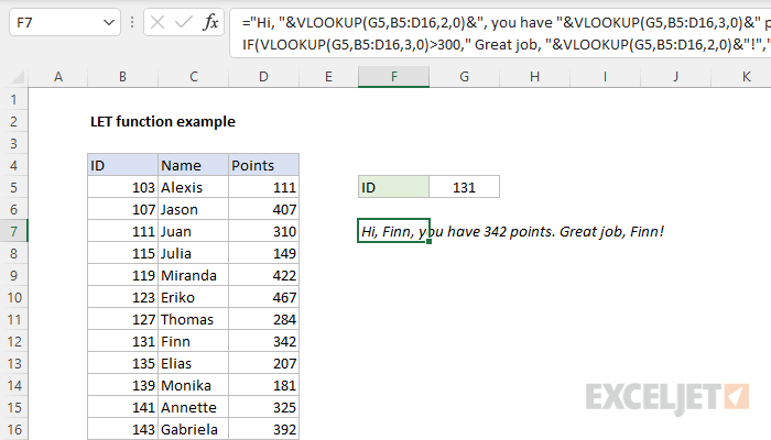
Finally, we need to join the first part of the message to the second part. The final formula is:
="Hi, "&VLOOKUP(G5,B5:D16,2,0)&", you have "&VLOOKUP(G5,B5:D16,3,0)&" points."&IF(VLOOKUP(G5,B5:D16,3,0)>300," Great job, "&VLOOKUP(G5,B5:D16,2,0)&"!","")
This formula works fine, but it’s getting a bit unwieldy. Notice we have four separate calls to VLOOKUP, and two of the four are exact duplicates:
Let’s use the LET function to slim down and simplify this formula.
Thinking about variables
To use the LET function, we need to think about variables . The main purpose of variables is to define a useful name that can be reused elsewhere in the formula code. In addition, when the value assigned to a variable is calculated , there is an opportunity to improve performance by reducing the number of times the calculation is performed. Using a variable also has the advantage of keeping a calculation in one place only, which reduces errors and the editing needed to keep multiple copies in sync.
Looking at the formula above, there are two obvious places where a named variable makes sense: the lookup for name , and the lookup for points . Both of these lookups appear twice in the formula, so this is a good opportunity to simplify.
Implementing LET
The basic pattern for implementing LET with two variables looks like this:
=LET(name1,value1,name2,value2,result)
Notice names and values appear in pairs – we declare name1 and assign value1 , then we declare name2 and assign value2 . Lastly, we add a result . The result is the final result returned by LET. This is typically a calculation, adjusted to use the declared variables.
In this case, we’ll use “name” for name1 , and “points” for name2 . To assign values to each variable, we’ll use the VLOOKUP function configured as shown below:
=VLOOKUP(G5,B5:D16,2,0) // look up name
=VLOOKUP(G5,B5:D16,3,0) // look up points
Putting this into the LET function, we begin like this:
=LET(name,VLOOKUP(G5,B5:D16,2,0),points,VLOOKUP(G5,B5:D16,3,0),
This defines the variables “name” and “points” and assigns values to both, based on the id in cell G5. Next, we need to add the calculation that determines a final result. We’ll start with the original formula above:
="Hi, "&VLOOKUP(G5,B5:D16,2,0)&", you have "&VLOOKUP(G5,B5:D16,3,0)&" points."&IF(VLOOKUP(G5,B5:D16,3,0)>300," Great job, "&VLOOKUP(G5,B5:D16,2,0)&"!","")
We could use this formula as-is, and it would run correctly, but it would defeat the purpose of using the LET function. To take advantage of LET, we need to replace the VLOOKUPs with the variables we’ve already declared, like this:
="Hi, "&name&", you have "&points&" points."&IF(points>300," Great job, "&name&"!","")
Now we need to add this code to the LET function as the last argument:
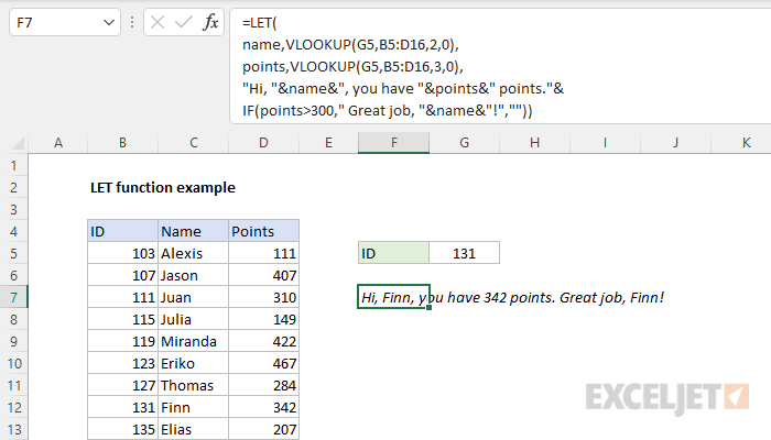
=LET(name,VLOOKUP(G5,B5:D16,2,0),points,VLOOKUP(G5,B5:D16,3,0),"Hi, "&name&", you have "&points&" points."&IF(points>300," Great job, "&name&"!",""))
This formula will return the same result as the original formula, but notice we only use VLOOKUP twice, instead of four times, and the calculation part of the formula is somewhat easier to read since we are using name and points as variables.
To improve readability, we can add line breaks (Alt + enter) like this:
=LET(
name,VLOOKUP(G5,B5:D16,2,0),
points,VLOOKUP(G5,B5:D16,3,0),
"Hi, "&name&", you have "&points&" points."&IF(points>300," Great job, "&name&"!",""))
You will see formatting like this frequently in formulas that use the LET function because it makes the formula easier to read, write, and edit. Here is the result in Excel. I’ve added one additional line break between part 1 and part 2 to keep everything on screen:
Note: you’ll need to expand the formula bar (control + shift + u) to see extra lines.
More readability
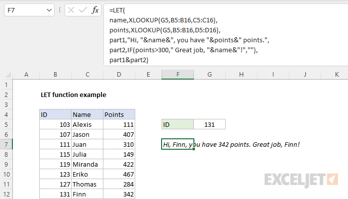
You are free to add more variables to LET if it helps you work with the formula more efficiently. For example, we could break the message into two parts, part1 and part2 , then join them together at the end like this:
=LET(
name,VLOOKUP(G5,B5:D16,2,0),
points,VLOOKUP(G5,B5:D16,3,0),
part1,"Hi, "&name&", you have "&points&" points.",
part2,IF(points>300," Great job, "&name&"!",""),
part1&part2)
This alternative won’t run any faster, but it can make the formula easier to read and create.
With XLOOKUP
One nice thing about LET is that it isolates calculation steps in a way that makes them easier to change. For example, although we’ve been using VLOOKUP to retrieve the name and points values we need, we can easily swap out VLOOKUP for XLOOKUP like this:
=LET(
name,XLOOKUP(G5,B5:B16,C5:C16),
points,XLOOKUP(G5,B5:B16,D5:D16),
part1,"Hi, "&name&", you have "&points&" points.",
part2,IF(points>300," Great job, "&name&"!",""),
part1&part2)
Notice we only changed the way name and points are defined. The rest of the formula did not change. Here is what this formula looks like in Excel with the formula bar expanded: