Explanation
This formula counts how many values are not in range of a fixed tolerance. The variation of each value is calculated with this:
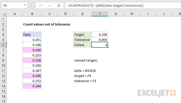
ABS(data-target)
Because the named range “data” contains 10 values, subtracting the target value in F4 will created an array with 10 results:
{0.001;-0.002;-0.01;0.003;0.008;0;-0.003;-0.01;0.002;-0.006}
The ABS function changes any negative values to positive:
{0.001;0.002;0.01;0.003;0.008;0;0.003;0.01;0.002;0.006}
This array is compared to the fixed tolerance in F5:
ABS(data-target)>tolerance
The result is an array or TRUE FALSE values, and the double negative changes these to ones and zeros. Inside SUMPRODUCT, the final array looks like this:
{0;0;1;0;1;0;0;1;0;1}
where zeros represent values within tolerance, and 1s represent values out of tolerance. SUMPRODUCT then sums the items in the array, and returns a final result, 4.
All values within tolerance
To return “Yes” if all values in a data range are within a given tolerance, and “No” if not, you can adapt the formula like this:
=IF(SUMPRODUCT(--(ABS(data-target)>tolerance)),"Yes","No")
If SUMPRODUCT returns any number greater than zero, IF will evaluate the logical test as TRUE. A zero result will be evaluated as FALSE.
Highlight values out of tolerance
You can highlight values out of tolerance with a conditional formatting rule based on a formula like this:
=ABS(B5-target)>tolerance
This page lists more examples of conditional formatting with formulas.
Explanation
The core of this formula is the ROUNDUP function. The ROUNDUP function works like the ROUND function except that when rounding, the ROUNDUP function will always round the numbers 1-9 up. In this formula, we use that fact to repeat values.
To supply a number to ROUNDUP, we are using this expression:
(COLUMN()-2)/$B4
Without a reference, COLUMN generates the column number of the cell it appears in, in this case 3 for cell C4.
The number 2 is simply an offset value, to account for the fact column C is column 3. We subtract 2 to normalize back to 1.
Cell B4 holds the value that represents the number of times to “repeat” a count. We’ve locked the column reference so that the repeat value remains fixed as the formula is copied across the table.
The normalized column number is divided by the repeat value and the result is fed into ROUNDUP as the number to round. For n umber of places, we use zero, so that rounding goes to the next integer.
Once the column count is evenly divisible by the repeat value, the count advances.
Rows instead of columns
If you need to count in rows, instead of columns, just adjust the formula like so:
=ROUNDUP((ROW()-offset)/repeat,0)
