Explanation
Data validation rules are triggered when a user adds or changes a cell value. This formula takes advantage of this behavior to provide a clever way for the user to switch between a short list of cities and a longer list of cities. In the worksheet shown, the data validation applied to C4 looks like this:
=IF(C4="See full list",long_list,short_list)
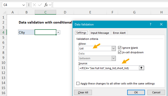
The IF function is configured to test the value in cell C4. When C4 contains the text “See full list”, IF returns the named range long_list. When C4 is empty or contains any other value IF returns the named range short_list.
Behavior
The user starts with the values in E6:E13 as seen below:
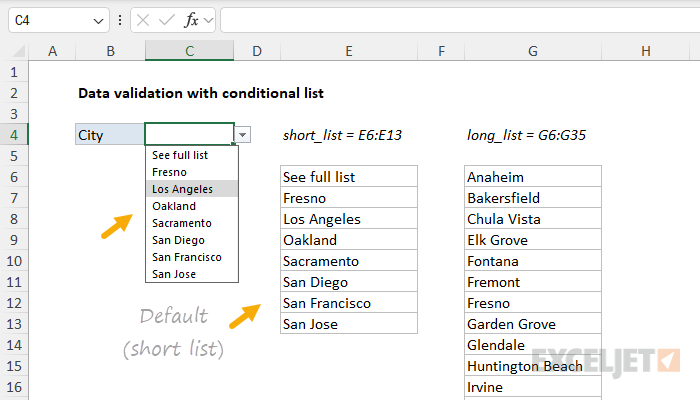
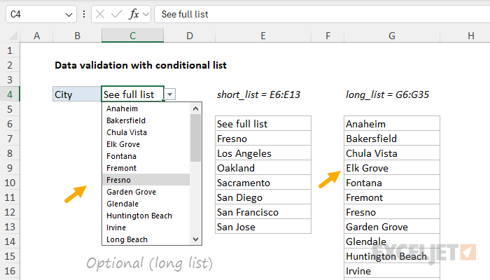
When the user selects “See full list”, they can select from the longer list of cities in G6:G35:
The named ranges used in the formula are not required, but they make the formula easier to read. If you are new to named ranges, this page provides a good overview .
Dependent dropdown lists
Expanding on the example above, you can create multiple dependent dropdown lists. For example, a user selects an item type of “fruit”, so they next see a list of fruits to select. If they first select “vegetable” they then see a list of vegetables. Click the image below for instructions and examples:
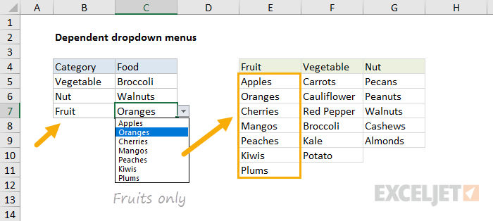
Data Validation Guide | Data Validation Formulas | Dependent Dropdown Lists
Explanation
In this example, the goal is to retrieve information about the lowest three estimates in the data shown. The problem is that there are some duplicate values in the estimate column. This means we will have some trouble trying to display the names of the 2nd and 3rd lowest suppliers because the tie values will cause INDEX to return the same name. One way to break ties like this is to add a helper column with values that have been adjusted, and then rank those values instead of the originals. In this example, the logic used to adjust values is random - the first duplicate value will “win”, but you can adjust the formula to use logic that fits your particular situation and use case.
COUNTIF with expanding reference
At the core, this formula uses the COUNTIF function and an expanding range to count occurrences of values. The expanding reference is used so that COUNTIFS returns a running count of occurrences , instead of a total count for each value:
COUNTIF($C$5:C5,C5)
Next, 1 is subtracted from the result (which makes the count of all non-duplicate values zero) and the result is multiplied by 0.01. This value is the “adjustment”, and is intentionally small so as not to materially impact the original value.
In the example shown, Metrolux and Diamond both have the same estimate of $5000. Since Metrolux appears first in the list, the running count of 5000 is 1 and is canceled out by subtracting 1, so the estimate remains unchanged in the helper column:
=C8+(COUNTIF($C$5:C8,C8)-1)*0.01
=C8+(1-1)*0.01
=C8+0
=C8
However, for Diamond, the running count of 5000 is 2, so the estimate is adjusted:
=C11+(COUNTIF($C$5:C11,C11)-1)*0.01
=C11+(2-1)*0.01
=C11+1*0.01
=C11+0.01
Finally, the adjusted values are used for ranking instead of the original values in columns G and H. The formula in G5 is:
=SMALL($D$5:$D$12,F5)
The formula in H5:
=INDEX($B$5:$B$12,MATCH(G5,$D$5:$D$12,0))
For a detailed explanation of these formulas, see this example .
Temporary helper column
If you don’t want to use a helper column in the final solution, you can use a helper column temporarily to get calculated values, then use Paste Special to convert values “in place” and delete the helper column afterward. This video demonstrates the technique.
