Explanation
In this example, the goal is to test a date to determine whether it is a workday. In Excel, you can use either the WORKDAY function or its more flexible sibling WORKDAY.INTL to accomplish this task.
WORKDAY function
The WORKDAY function calculates a date in the future or past that is, by definition, a workday. WORKDAY automatically excludes weekends (Saturday and Sunday) and can optionally exclude holidays. WORKDAY accepts 3 arguments: start_date , days , and (optionally) holidays . The generic syntax looks like this:
=WORKDAY(start_date,days,[holidays])
For example, if we provide WORKDAY with the date May 31, 2024 (a Friday), and ask for a workday 1 day in the future, WORKDAY skips Saturday and Sunday and returns June 3, 2024:
=WORKDAY("31-May-2024",1) // returns "3-June-2024"
In this example, we are not providing holidays. If we have a list of dates that are holidays we can provide them like this:
=WORKDAY("31-May-2024",1,holidays) // returns "3-June-2024"
Where “holidays” is a previously defined named range , or a simple range like G5:G7, usually entered as an absolute reference like $G$5:$G$7 to prevent changes when the formula is copied.
Testing for a workday
Since in this problem we want to check a single date and get a TRUE or FALSE result, we would ideally use WORKDAY with days set to zero in a simple formula like this:
=WORKDAY(date,0,holidays)=B5
However, this doesn’t work, since WORKDAY will not evaluate a date when days is zero. It always returns the original start date, even if it is a weekend or holiday. The solution is to supply the start_date as a simple calculation that subtracts 1 like this:
=WORKDAY(B5-1,1,holidays)=B5
This causes WORKDAY to step back one day, then add 1 day to the result, taking into account weekends and holidays. Effectively, we are “tricking” WORKDAY into evaluating the original date as the start_date . When the date falls on a weekend or holiday, WEEKDAY will automatically adjust the date forward to the next working day. If the date is a workday, it will remain unchanged. Then we compare the original start date in cell B5 to the result of the WORKDAY function. If the dates are the same (i.e. the result from WORKDAY is the same as the date in B5) we know we have a workday and the formula returns TRUE. If not, WORKDAY has shifted the date (which means it is a non-working day) and the formula returns FALSE. This is the formula used in cell D5 of the worksheet shown above.
Shading non-workdays with conditional formatting
In the worksheet shown, we are also shading non-workdays in gray with conditional formatting , triggered by this formula:
=WORKDAY(B5-1,1,holidays)<>B5
This formula is almost the same, but notice that we are comparing the result from WORKDAY with the original date using the “not equal to” operator ("<>") instead of the “equal to” ("=") operator. This reverses the operation of the formula so that it returns TRUE when a date is not a workday and FALSE when a date is a workday. We do this because we want to shade non-workdays .
Ensure a calculated date falls on a workday
If you are returning a date with another formula and want to make sure the date is a workday, you can use a formula like this:
=WORKDAY(calculated_date-1,1,holidays)
The idea is the same as above - we subtract one day from the date, then ask WORKDAY to give us the next working day.
Note: if you need to evaluate workdays with a custom workweek schedule, where weekends are not Saturday and Sunday, use the more flexible WORKDAY.INTL function.
Explanation
In this example, the goal is to get the total number of days in a month based on any date in the month. This problem can be solved by combining the DAY function with the EOMONTH function.
The EOMONTH function
The EOMONTH function returns the last day of the month, a given number of months in the past or future. For example, with a start date of June 15, 2024, EOMONTH will return the following results with months set to -1,0, and 1:
=EOMONTH("15-Jun-2024",-1) // returns 31-May-2024
=EOMONTH("15-Jun-2024",0) // returns 30-Jun-2024
=EOMONTH("15-Jun-2024",1) // returns 31-Jul-2024
Note that the start date remains the same, but the month varies. Negative months cause EOMONTH to move back in time, and positive months move forward, but the result is always the end of the month. Providing months as zero (0) will move EOMONTH to the end of the “current” month, relative to the date provided.
The DAY function
The DAY function returns the day component of any date, for example:
=DAY("15-Jun-2019") // returns 15
=DAY("7-Aug-2021") // returns 7
=DAY("23-Nov-2023") // returns 23
Note that in each case DAY returns the day value for the date.
Combining DAY and EOMONTH
Since, by definition, the last day of a month is equal to the number of days in the month, we can use DAY with EOMONTH to calculate the number of days in a month. In the worksheet shown, the formula in cell D5 looks like this:
=DAY(EOMONTH(B5,0))
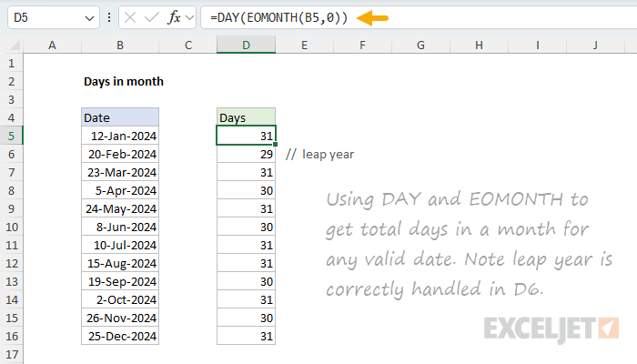
Working from the inside out, the EOMONTH function returns the last day of the month using the date in B5 as a starting point. Notice that the months argument is provided as zero so that we stay in the same month. Next, the shifted date is returned to the DAY function, which returns the day part of the date as a final result. Since the last day in January is the 31st, the final result is 31:
=DAY(EOMONTH("12-Jan-2024",0))
=DAY("31-Jan-2024")
=31
As the formula is copied down, the process is repeated for each date in column B.
Days in the Current Month
To get the number of days in the current month (today’s month), you can use the same approach but replace the date reference with the TODAY function :
=DAY(EOMONTH(TODAY(),0))
This formula will automatically update each day to show the total number of days in whatever month it currently is. For example, if today is June 21, 2025, the formula will return 30 (since June has 30 days). If you open the same worksheet in July, it will automatically return 31. The formula works exactly the same way as the main example:
=DAY(EOMONTH(TODAY(),0))
=DAY(EOMONTH("21-Jun-2025",0))  // TODAY() returns current date
=DAY("30-Jun-2025")             // EOMONTH finds last day of June
=30                             // DAY extracts the day number
This approach is useful in reports and dashboards that need to display current-month information. Since TODAY recalculates whenever the worksheet recalculates, this formula will always reflect the correct number of days for the current month.
Explanation
In the worksheet shown, column B contains 12 dates. The goal is to calculate the next working day after each date, taking into account weekends (Saturday and Sunday) and the holidays listed in column F. In other words, the formula should automatically skip weekends and any dates defined as non-working days.
WORKDAY function
The WORKDAY function takes a date and returns the next working day n days in the future or past. You can use WORKDAY to calculate things like ship dates, delivery dates, and completion dates that need to take into account working and non-working days. The generic syntax for WORKDAY looks like this:
=WORKDAY(start_date,days,[holidays])
Where days is a number (n) and holidays is an optional range that contains non-working dates. For this problem, we want the next working day, so we provide 1 for days . The formula in D5, copied down, looks like this:
=WORKDAY(B5,1,holidays)
Where holidays is the named range F5:F15, which contains days that should be excluded. The WORKDAY function is fully automatic. Given a valid date, it will add days to the date, skipping weekends and holidays. Named ranges behave like absolute references by default, so the range will not change as the formula is copied down. Without a named range, you will need to lock the reference like this:
=WORKDAY(B5,1,$F$5:$F$15)
As the formula is copied down, it returns the next business day after the starting date in column B. Saturdays and Sundays are automatically skipped, as well as any dates that appear in the range F5:F15.
Current date or next workday
There may be situations where you want to return the current date when it’s a working day or the next working date if not. To do this, you can adjust the formula like so:
=WORKDAY(B5-1,1,holidays)
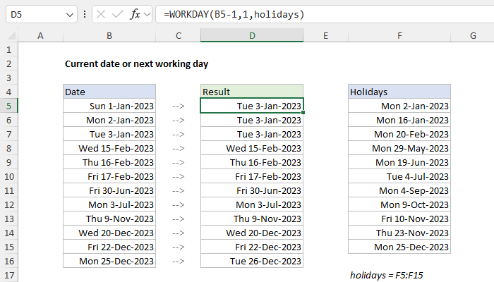
Here, we first subtract 1 day from the date inside the WORKDAY function, then feed that date to WORKDAY as the start_date . WORKDAY then moves forward one day to the original date and checks the result. If the original date is a working day, WORKDAY returns the date unchanged. Otherwise, WORKDAY will continue to move forward one day at a time, skipping weekends and holidays along the way, until it finds a valid workday. You can see the result in the worksheet above.
Custom weekends
The WORKDAY function defines a weekend as Saturday and Sunday only. If you need more flexibility on which days of the week are considered weekends or working days, use the WORKDAY.INTL function instead. For example, to calculate the next working day for this example with a standard work week of Monday-Thursday, where weekend days are Friday, Saturday, and Sunday, you can use WORKDAY.INTL like this:
=WORKDAY.INTL(B5,1,"0000111",holidays)
WORKDAY.INTL includes an extra argument called weekend that can be provided as a string of 1s and 0s like “0000111”. In this scheme, a 1 indicates a weekend and a 0 indicates a workday. For more details, see How to use the WORKDAY.INTL function .
Explanation
Working from the inside out, EDATE first calculates a date 6 months in the future. In the example shown, that date is December 24, 2015.
Next, the formula subtracts 1 day to get December 23, 2015, and the result goes into the WORKDAY function as the start date, with days = 1, and the range B9:B11 provided for holidays.
WORKDAY then calculates the next business day one day in the future, taking into account holidays and weekends.
If you need more flexibility with weekends, you can use WORKDAY.INTL.
