Purpose
Return value
Syntax
=DATEDIF(start_date,end_date,unit)
- start_date - Start date in Excel date serial number format.
- end_date - End date in Excel date serial number format.
- unit - The time unit to use (years, months, or days).
Using the DATEDIF function
The DATEDIF function is designed to calculate the difference between two date values in years, months, or days. The result from DATEDIF is a number that corresponds to the time unit requested. DATEDIF is a versatile function that can be used in financial analysis, project planning, age calculation, and other scenarios that need to calculate time intervals in days, months, or years.
The status of DATEDIF in Excel is somewhat mysterious. DATEDIF (Date + Dif) is a “compatibility” function that comes from Lotus 1-2-3 way back in the 1990s. Although it’s available in all Excel versions since that time, it will not autocomplete in the formula bar, and Excel will not help you fill in arguments for DATEDIF like other functions. In the immortal words of the late, great Chip Pearson: DATEDIF is treated as the drunk cousin of the Formula family. Excel knows it lives a happy and useful life, but will not speak of it in polite conversation. Yet DATEDIF remains an important function for problems that involve calculating the time between two dates.
DATEDIF and time units
The DATEDIF function can calculate the time between a start date and an end date in years, months, or days. The desired interval is specified with the unit argument, which is supplied as text. The table below shows the available unit values and the results for each. Time units can be provided in upper or lower case (i.e. “ym” is equivalent to “YM”).
| Unit | Result |
|---|---|
| “y” | Difference in complete years |
| “m” | Difference in complete months |
| “d” | Difference in days |
| “md” | Difference in days, ignoring months and years |
| “ym” | Difference in months, ignoring years |
| “yd” | Difference in days, ignoring years |
Example 1 - Basic usage
The basic syntax for DATEDIF looks like this:
=DATEDIF(start_date,end_date,unit)
The formulas below show how to use DATEDIF to calculate complete years, months, and days between January 1, 2022, and March 1, 2024. Notice the formulas are the same except for the unit:
=DATEDIF("1-Jan-2022","1-Mar-2024","y") // returns 2
=DATEDIF("1-Jan-2022","1-Mar-2024","m") // returns 26
=DATEDIF("1-Jan-2022","1-Mar-2024","d")// returns 790
The results are as follows:
- There are 2 complete years between the dates. Although there are 26 months between the two dates, DATEDIF ignores the extra 2 months since it’s not a complete year.
- There are 26 months between the dates. DATEDIF will always round down to the nearest whole month but in this case, the day is the same in the start and end dates, so no rounding occurs.
- There are 790 days between the dates.
DATEDIF requires the start date followed by the end date. If you reverse the dates, DATEDIF returns a #NUM! error.
Example 2 - Difference in days
The DATEDIF function can calculate the difference between dates in days in three different ways: (1) total days, (2) days ignoring years, and (3) days ignoring months and years. The screenshot below shows all three methods, with a start date of June 15, 2015, and an end date of September 15, 2021:

The formulas used for these calculations are as follows:
=DATEDIF(B5,C5,"d") // total days
=DATEDIF(B6,C6,"yd") // days ignoring years
=DATEDIF(B7,C7,"md") // days ignoring months and years
Note that because Excel dates are just large serial numbers , the first formula does not need DATEDIF and could be written as simply the end date minus the start date:
=C5-B5 // end-start = total days
Note: You could also use the newer DAYS function to calculate a difference in days.
Example 3 - Difference in months
The DATEDIF function can calculate the difference between dates in months in two different ways: (1) total complete months, (2) complete months ignoring years. The screenshot below shows both methods, with a start date of June 15, 2015, and an end date of September 15, 2021:

=DATEDIF(B5,C5,"m") // complete months
=DATEDIF(B6,C6,"ym") // complete months ignoring years
DATEDIF always rounds months down to the nearest whole month. This means DATEDIF will round months down even when it is very close to the next whole month. In addition, DATEDIF may not work as expected when start and end dates land a the end of a month. For a detailed explanation of calculating months between dates with several alternative formulas, see this example .
Example 4 - Difference in years
The DATEDIF function can calculate the difference between dates in complete years with just one method, shown below:

=DATEDIF(B5,C5,"y") // complete years
=DATEDIF(B6,C6,"y") // complete years
=YEARFRAC(B7,C7) // fractional  years with YEARFRAC
Notice in row 6 that the difference is almost 6 years, but not quite. Because DATEDIF only calculates complete years, the result is still 5. In row 7 we use the YEARFRAC function to calculate a more accurate result.
Example 5 - Age from birthday
The DATEDIF function can be used together with the TODAY function to calculate a current age from a birth date. With a birth date in A1, the generic formula is:
=DATEDIF(A1,TODAY(),"y")
You can see this formula implemented in the worksheet below:

Note: The screen above was created on November 24, 2020, so the calculated ages will seem too young over time. However, because we are using the TODAY function, this formula will recalculate and the ages will be correct each time the workbook is opened. Download the workbook and read a complete explanation on this page .
Example 6 - years, months, and days between dates
You can use the DATEDIF function to calculate the years, months, and days between dates, as seen in the workbook below. The formula in cell E5, copied down, looks like this:
=DATEDIF(B5,C5,"y")&" years, "&DATEDIF(B5,C5,"ym")&" months, " &DATEDIF(B5,C5,"md")&" days"
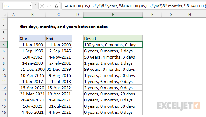
This is a good example of how DATEDIF’s ability to calculate months ignoring years and days ignoring years and months can be useful. You can find a full explanation and download the workbook on this page .
Notes
- Excel will not help you fill in the DATEDIF function like other functions.
- DATEDIF will throw a #NUM error if start_date is greater than the end_date . If you are working with a more complex formula where start dates and end dates may be unknown, or out of bounds, you can trap the error with the IFERROR function .
- Microsoft recommends not using the “MD” value for unit because it “may result in a negative number, a zero, or an inaccurate result”.
Purpose
Return value
Syntax
=DATEVALUE(date_text)
- date_text - A valid date in text format.
Using the DATEVALUE function
Sometimes, dates in Excel appear as text values that are not recognized as proper dates. The DATEVALUE function is meant to convert a date represented as a text string into a valid Excel date . Proper Excel dates are more useful than text dates since they can be formatted as a date, and directly manipulated with other formulas.
The DATEVALUE function takes just one argument, called date_text . If date_text is a cell address, the value of the cell must be text. If date_text is entered directly into the formula it must be enclosed in quotes.
Examples
To illustrate how the DATEVALUE function works, the formula below shows how the text “3/10/1975” is converted to the date serial number 27463 by DATEVALUE:
=DATEVALUE("3/10/1975") // returns 27463
Note that DATEVALUE returns a serial number, 27463, which represents March 10, 1975 in Excel’s date system. A date number format must be applied to display this number as a date.
In the example shown, column B contains dates entered as text values, except for B15, which contains a valid date. The formula in C5, copied down, is:
=DATEVALUE(B5)
Column C shows the number returned by DATEVALUE, and column D shows the same number formatted as a date . Notice that Excel makes certain assumptions about missing day and year values. Missing days become the number 1, and the current year is used if there is no year value available.
Alternative formula
Notice that the DATEVALUE formula in C15 fails with a #VALUE! error, because cell B15 already contains a valid date. This is a limitation of the DATEVALUE function. If you have a mix of valid and invalid dates, you can try the simple formula below as an alternative:
=A1+0
The math operation of adding zero will cause Excel will try to coerce the value in A1 to a number. If Excel can parse the text into a proper date it will return a valid date serial number. If the date is already a valid Excel date (i.e. a serial number), adding zero will have no effect, and generate no error.
Notes
- DATEVALUE will return a #VALUE error if date_text refers does not contain a date formatted as text.
Explanation
Working from the inside out, we use the DATEDIF function to calculate how many complete years are between the original anniversary date and the “as of” date, where the as of date is any date after the anniversary date:
DATEDIF(B5,C5,"y")
Note: in this case, we are arbitrarily fixing the “as of” date as June 1, 2017 in all examples.
Because we are interested in the next anniversary date, we add 1 to the DATEDIF result, then multiply by 12 to convert to years to months.
Next, the month value goes into the EDATE function, with the original date from column B. The EDATE function rolls the original date forward by the number of months given in the previous step which creates the next upcoming anniversary date.
As of today
To calculate the next anniversary as of today, use the TODAY() function for the “as of” date:
=EDATE(date,(DATEDIF(date,TODAY(),"y")+1)*12)
