Explanation
This formula relies on a specific behavior of INDEX — although it seems that INDEX returns the value at a particular location, it actually returns a reference to the location. In most formulas, you wouldn’t notice the difference – Excel simply evaluates the reference and returns the value. This formula uses this feature to construct a dynamic range based on worksheet input.
Inside the sum function, the first reference is simply the first cell in the range that covers all possible cells:
=SUM(C5:
To get the last cell, we use INDEX. Here, we give INDEX the named range “data”, which is the maximum possible range of values, and also the values from J5 (rows) and J6 (columns). INDEX doesn’t return a range, it only returns a single cell at that location, E9 in the example:
INDEX(data,J5,J6) // returns E9
The original formula is reduced to:
=SUM(C5:E9)
which returns 300, the sum of all values in C5:E9.
The formula in J8 is almost the same but uses AVERAGE instead of SUM to calculate an average. When a user changes values in J5 or J6 the range is updated, and new results are returned.
Alternative with OFFSET
You can build a similar formula with the OFFSET function , shown below:
=SUM(OFFSET(C5,0,0,J5,J6)) // sum
=AVERAGE(OFFSET(C5,0,0,J5,J6)) // average
OFFSET is designed to return a range, so the formulas are perhaps simpler to understand. However, OFFSET is a volatile function and can cause performance problems when used in larger, more complex worksheets.
Explanation
This page shows an example of a dynamic named range created with the INDEX function together with the COUNTA function. Dynamic named ranges automatically expand and contract when data is added or removed. They are an alternative to using an Excel Table , which also resizes as data is added or removed.
The INDEX function returns the value at a given position in a range or array. You can use INDEX to retrieve individual values or entire rows and columns in a range. What makes INDEX especially useful for dynamic named ranges is that it actually returns a reference. This means you can use INDEX to construct a mixed reference like $A$1:A100.
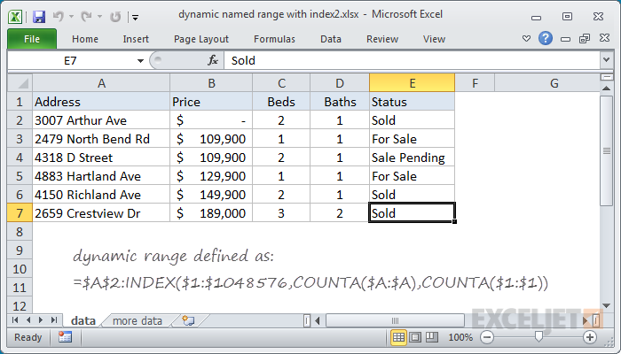
In the example shown, the named range “data” is defined by the following formula:
=$A$2:INDEX($A:$A,COUNTA($A:$A))
which resolves to the range $A$2:$A$10.
How this formula works
Note first that this formula is composed of two parts that sit on either side of the range operator (:). On the left, we have the starting reference for the range, hard coded as:
$A$2
On the right is the ending reference for the range, created with INDEX like this:
INDEX($A:$A,COUNTA($A:$A))
Here, we feed INDEX all of column A for the array, then use the COUNTA function to figure out the “last row” in the range. COUNTA works well here because there are 10 values in column A, including a header row. COUNTA therefore returns 10, which goes directly into INDEX as the row number. INDEX then returns a reference to $A$10, the last used row in the range:
INDEX($A:$A,10) // resolves to $A$10
So, the final result of the formula is this range:
$A$2:$A$10
A two-dimensional range
The above example works for a one-dimensional range. To create a two-dimensional dynamic range where the number of columns is also dynamic, you can use the same approach, expanded like this:
=$A$2:INDEX($1:$1048576,COUNTA($A:$A),COUNTA($1:$1))
As before, COUNTA is used to figure out the “lastrow”, and we use COUNTA again to get the “lastcolumn”. These are supplied to INDEX as row_num and column_num respectively.
However, for the array, we supply the full worksheet, entered as all 1048576 rows, which allows INDEX to return a reference in a 2D space.
Determining the last row
There are several ways to determine the last row (last relative position) in a set of data, depending on the structure and content of the data in the worksheet:
- Last row in mixed data with blanks
- Last row in mixed data with no blanks
- Last row in text data
- Last row in numeric data
