Purpose
Return value
Syntax
=DETECTLANGUAGE(text)
- text - A sample of the language as a text string.
Using the DETECTLANGUAGE function
The DETECTLANGUAGE figures the language for a given text string. The result from DETECTLANGUAGE is a short language code indicating the language. For example, if the language is English, the result is “en”; if the language is French, the result is “fr”; if the language is Japanese, the result is “ja”, and so on. Some of these codes are intuitive, but some aren’t. See below for a list of common language codes. DETECTLANGUAGE only accepts one argument, text, so the syntax is very simple and looks like this:
=DETECTLANGUAGE(text)
Typically, the text is supplied as a cell reference like A1, but it can also be hardcoded as a string like “apple”.
The DETECTLANGUAGE function uses Microsoft Translation Services, so it requires an internet connection.
Basic Example
To use the DETECTLANGUAGE function, simply provide some text. For example, if we give DETECTLANGUAGE the word “apple”, it “detects” English and returns “en”:
=DETECTLANGUAGE("apple") // returns "en"
Likewise, if we give DETECTLANGUAGE the word for “apple” in four languages (French, Italian, German, and Spanish), it returns the four corresponding language codes: “fr,” “it,” “de,” and “es.”
=DETECTLANGUAGE("pomme")  //  returns "fr"
=DETECTLANGUAGE("mela")  //  returns "it"
=DETECTLANGUAGE("Apfel")  //  returns "de"
=DETECTLANGUAGE("manzana")  //  returns "es"
Note that DETECTLANGUAGE always returns a language code like “en”, “it”, “de”, “es”, etc. The TRANSLATE function supports over 100 languages, so there are many potential codes. See below for a list of common languages and codes.
Example: Get language codes
In the worksheet below, we have text for “Is there a coffee shop around here?” in 12 languages. The goal is to determine the language codes based on the text in column B. The formula in D8, copied down, looks like this:
=DETECTLANGUAGE(B5)
As the formula is copied down the column, DETECTLANGUAGE returns a language code for each text string, as seen in column D below:

Note that the DETECTLANGUAGE function is dynamic. If any of the text in column B is changed to a different language, TRANSLATE will return a new language code.
Example: Get language names
Getting language codes automatically is great, but you probably want to know how to get an actual language name. To do that, you will want to set up a lookup table in your worksheet with columns for the language code and the language name. In the worksheet below, we have defined an Excel Table called “languages” like this:

Then we can use the XLOOKUP function to get the correct language for a given code, as seen in column E of the worksheet below. The formula in cell E5 looks like this:
=XLOOKUP(D5,languages[Code],languages[Language])
The inputs to XLOOKUP are as follows:
- lookup_value - D5
- lookup_array - languages[Code]
- return_array - languages[Language]

If you want to look up the language name from the code in one step, you can combine the formulas above into one formula like this:
=XLOOKUP(DETECTLANGUAGE(B5),languages[Code],languages[Language])
In this formula, DETECTLANGUAGE returns a language code to XLOOKUP as the lookup value, and XLOOKUP uses the code to get the language name in a single step.
Excel Tables make it possible to use “structured references” in formulas, like languages[Code] and languages[Language]. One advantage to structured references is that we don’t need to lock any references in a formula like this. To learn more see our Excel Table guide .
Codes for common languages
The below shows language codes for some common languages that can be used with the TRANSLATE function. Note that some languages, like Portuguese, have more than one variant. For example, the code “pt” specifies Portuguese for Brazil, while “pt-pt” specifies Portuguese for Portugal.
| Language | Code | Notes |
|---|---|---|
| Arabic | ar | |
| Chinese | zh-Hans | Simplified |
| Czech | cs | |
| Danish | da | |
| Dutch | nl | |
| English | en | |
| Finnish | fi | |
| French | fr | |
| German | de | |
| Hindi | hi | |
| Indonesian | id | |
| Italian | it | |
| Japanese | ja | |
| Korean | ko | |
| Norwegian | nb | Bokmål |
| Polish | pl | |
| Portuguese | pt | Brazilian |
| Spanish | es | |
| Swedish | sv | |
| Thai | th | |
| Vietnamese | vi |
The DETECTLANGUAGE function supports over 130 languages. You can find the full list of supported languages here .
Notes
- DETECTLANGUAGE always returns a language code as text.
- If the text is an empty string (""), DETECTLANGUAGE also returns an empty string.
- If the internet is not available, you may see a #CONNECT! error.
- Use the TRANSLATE function to translate text to another language.
Purpose
Return value
Syntax
=DROP(array,[rows],[col])
- array - The source array or range.
- rows - [optional] Number of rows to drop.
- col - [optional] Number of columns to drop.
Using the DROP function
The DROP function returns a subset of a given array by “dropping” rows and columns. The number of rows and columns to remove is provided by separate rows and columns arguments. Rows and columns can be dropped from the start or end of the given array. When positive numbers are provided for rows or columns , DROP removes values from the start or top of the array. Negative numbers remove values from the end or bottom of the array.
The DROP function takes three arguments: array , rows , and columns . Array is required, along with at least one value for rows or columns . Array can be a range or an in-memory array from another formula. Rows and columns can be negative or positive. Positive numbers remove values from the start of the array ; negative numbers remove values from the end of the array . Both rows and columns default to zero: if no value is supplied, DROP will return all rows/columns in the result.
Basic usage
To use DROP, provide an array or range , and numbers for rows and/or columns:
=DROP(array,3) // drop first 3 rows
=DROP(array,,3) // drop first 3 columns
=DROP(array,3,2) // drop first 3 rows and 2 columns
Notice in the second example above, no value is provided for rows.
Drop from start
To remove rows or columns from the start of a range or array, provide positive numbers for rows and columns. In the worksheet below, the formula in F3 is:
=DROP(B3:D11,6) // drop first 6 rows
The DROP function removes the first 6 rows from B3:D11 and returns the resulting array.
The second formula in F8 is:
=DROP(B3:D11,5,1) // drop first 5 rows and column 1
The DROP function removes the first 5 rows and column 1 from B3:D11 and returns the result.
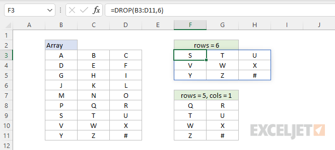
Notice that if a value for rows or columns is not provided, DROP returns all rows or columns. For example, in the first formula above, a value for columns is not provided and DROP returns all 3 columns as a result. In other words, rows and columns both default to zero.
Drop from end
To remove values from the end of an array, provide negative numbers for rows and columns . In the worksheet below, the formula in cell F3 is:
=DROP(B3:D11,-6)
With a negative 6 for rows , DROP removes the last 6 rows from B3:D11.
The formula in F8 is:
=DROP(B3:D11,-5,-1)
With a negative 5 for rows and a negative 1 for columns , DROP removes the last 5 rows and the last 1 column from B3:D11 and returns the resulting array to cell F8.
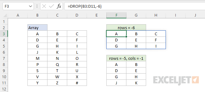
Notice in the first example, no value for columns is given and DROP returns all columns as a result.
DROP vs. TAKE
The DROP and TAKE functions both return a subset of an array, but they work in opposite ways. While the DROP function removes specific rows or columns from an array, the TAKE function extracts specific rows or columns from an array:
=DROP(array,1) // remove first row
=TAKE(array,1) // get first row
Which function to use depends on the situation.
Notes
- Rows and columns are both optional, but at least one must be provided.
- If rows or columns is zero, DROP returns all rows/columns.
- If rows > total rows, DROP returns a #VALUE! error
- If columns > total columns, DROP returns a #VALUE! error
