To make a dynamic chart that automatically skips empty values, you can use dynamic named ranges created with formulas. When a new value is added, the chart automatically expands to include the value. If a value is deleted, the chart automatically removes the label.
In the chart shown, data is plotted in one series. Values come from a named range called “values”, defined with the formula provided below:
=$C$4:INDEX($C$4:$C$30,COUNT($C$4:$C$30)) // values
Axis labels come from a named range called “groups”, defined with this formula:
=$B$4:INDEX($B$4:$B$30,COUNT($C$4:$C$30)) // groups
This page explains dynamic named ranges created with INDEX in more detail.
How to make this chart
Create a normal chart, based on the values shown in the table. If you include all rows, Excel will plot empty values as well.
Using the name manager (control + F3) define the name “groups”. In the “refers to” box, use a formula like this:
=$B$4:INDEX($B$4:$B$30,COUNT($C$4:$C$30))
- Define a name for “values” with the same process, using this formula:
=$C$4:INDEX($C$4:$C$30,COUNT($C$4:$C$30))
- Edit the data series with the Select data command. For series values, use the defined name “values” with the sheet name prepended:
=Sheet1!values

For category labels, use the defined name “groups” with the sheet name prepended:
=Sheet1!groups

- Click OK twice to save changes and exit the Select Data dialog.
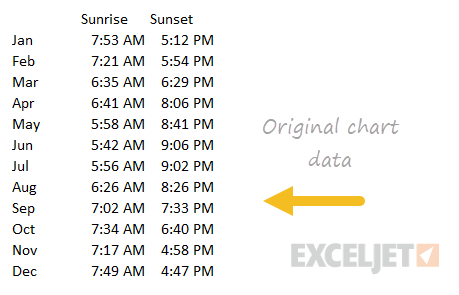
This chart is an example of a column chart that uses a “floating bar” technique to plot daylight hours on the chart in way that makes the bars look like the are floating above the horizontal axis. The trick in this case is to create three helper columns that do not exist in the original data: daylight, evening, and hrs. The video here walks through this process.
Original data
Data with helper columns

