Explanation
This page shows an example of a dynamic named range created with the INDEX function together with the COUNTA function. Dynamic named ranges automatically expand and contract when data is added or removed. They are an alternative to using an Excel Table , which also resizes as data is added or removed.
The INDEX function returns the value at a given position in a range or array. You can use INDEX to retrieve individual values or entire rows and columns in a range. What makes INDEX especially useful for dynamic named ranges is that it actually returns a reference. This means you can use INDEX to construct a mixed reference like $A$1:A100.
In the example shown, the named range “data” is defined by the following formula:
=$A$2:INDEX($A:$A,COUNTA($A:$A))
which resolves to the range $A$2:$A$10.
How this formula works
Note first that this formula is composed of two parts that sit on either side of the range operator (:). On the left, we have the starting reference for the range, hard coded as:
$A$2
On the right is the ending reference for the range, created with INDEX like this:
INDEX($A:$A,COUNTA($A:$A))
Here, we feed INDEX all of column A for the array, then use the COUNTA function to figure out the “last row” in the range. COUNTA works well here because there are 10 values in column A, including a header row. COUNTA therefore returns 10, which goes directly into INDEX as the row number. INDEX then returns a reference to $A$10, the last used row in the range:
INDEX($A:$A,10) // resolves to $A$10
So, the final result of the formula is this range:
$A$2:$A$10
A two-dimensional range
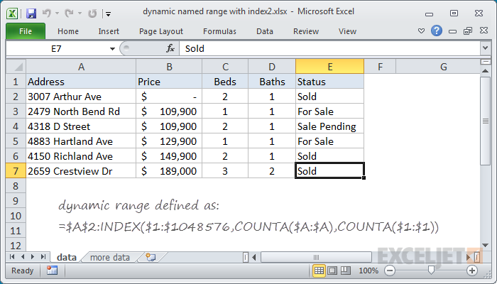
The above example works for a one-dimensional range. To create a two-dimensional dynamic range where the number of columns is also dynamic, you can use the same approach, expanded like this:
=$A$2:INDEX($1:$1048576,COUNTA($A:$A),COUNTA($1:$1))
As before, COUNTA is used to figure out the “lastrow”, and we use COUNTA again to get the “lastcolumn”. These are supplied to INDEX as row_num and column_num respectively.
However, for the array, we supply the full worksheet, entered as all 1048576 rows, which allows INDEX to return a reference in a 2D space.
Determining the last row
There are several ways to determine the last row (last relative position) in a set of data, depending on the structure and content of the data in the worksheet:
- Last row in mixed data with blanks
- Last row in mixed data with no blanks
- Last row in text data
- Last row in numeric data
Explanation
Dynamic ranges are also known as expanding ranges because they automatically expand and contract to accommodate new or deleted data. You can see a video demo of this approach here . This formula uses the OFFSET function to generate a range that expands and contracts by adjusting height and width based on a count of non-empty cells:
=OFFSET(B5,0,0,COUNTA($B$5:$B$100),COUNTA($B$4:$Z$4))
The first argument in OFFSET represents the first cell in the data (the origin), which in this case is cell B5. The next two arguments are offsets for rows and columns and are supplied as zero.
The last two arguments represent height and width. Height and width are generated on the fly by using COUNTA, which makes the resulting reference dynamic.
For height, we use the COUNTA function to count non-empty values in the range B5:B100. This assumes no blank values in the data, and no values beyond B100. COUNTA returns 6.
For width, we use the COUNTA function to count non-empty values in the range B5:Z5. This assumes no header cells, and no headers beyond Z5. COUNTA returns 6.
At this point, the formula looks like this:
=OFFSET(B5,0,0,6,6)
With this information, OFFSET returns a reference to B5:G10, which corresponds to a range 6 rows height by 6 columns across.
Note: The ranges used for height and width should be adjusted to match the worksheet layout.
Variation with full column/row references
You can also use full column and row references for height and width like so:
=OFFSET($B$5,0,0,COUNTA($B:$B)-2,COUNTA($4:$4))
Note that height is being adjusted with -2 to take into account header and title values in cells B4 and B2. The advantage of this approach is the simplicity of the ranges inside COUNTA. The disadvantage comes from the huge size full columns and rows — care must be taken to prevent errant values outside the range, as they can easily throw off the count.
Determining the last row
There are several ways to determine the last row (last relative position) in a set of data, depending on the structure and content of the data in the worksheet:
- Last row in mixed data with blanks
- Last row in mixed data with no blanks
- Last row in text data
- Last row in numeric data
