Purpose
Return value
Syntax
=EDATE(start_date,months)
- start_date - Start date as a valid Excel date.
- months - Number of months before or after start_date.
Using the EDATE function
The EDATE function returns a date on the same day of the month, n months before or after a start date. You can use EDATE to generate expiration dates, contract dates, due dates, anniversary dates, retirement dates, and other dates that derive from a start date. EDATE returns a serial number corresponding to a date . To display the result as a date, apply a number format of your choice .
The EDATE function takes two arguments , start_date and months :
- start_date - a valid Excel date to use as the starting point.
- months - a whole number that specifies how many months to move. Use a positive number of months to get a date in the future and a negative number for a date in the past.
Note: The EDATE function returns the same day of the month. If you want to get the last day of a month, use the EOMONTH function .
The EDATE function explained
With a given start date, EDATE returns a new date by adding the number of months provided. To illustrate how EDATE works, assume we want to create dates for the first day of each quarter, starting from January 1, 2024. We can do this with the following formulas:
=EDATE("1-Jan-2024",0) // returns 1-Jan-2024
=EDATE("1-Jan-2024",3) // returns 1-Apr-2024
=EDATE("1-Jan-2024",6) // returns 1-Jul-2024
=EDATE("1-Jan-2024",9) // returns 1-Oct-2024
The first formula does not change the date since months is zero. The second formula adds 3 months, the third formula adds 6 months, and the fourth formula adds 9 months to the date. In all cases, EDATE returns the 1st of the month since the start date is also the 1st. Of course, in most real-life scenarios, you will not hardcode dates into formulas like this. You will instead use cell references. If we enter the date January 1, 2024, in cell A1, the same formulas look like this:
=EDATE(A1,0) // returns 1-Jan-2024
=EDATE(A1,3) // returns 1-Apr-2024
=EDATE(A1,6) // returns 1-Jul-2024
=EDATE(A1,9) // returns 1-Oct-2024
The results are the same. And if the date in A1 is changed, EDATE will generate new dates. You can use negative numbers for months to create dates before the start date. With the same date in A1, the formulas below return dates that are 3, 6, 9, and 12 months before January 1, 2024:
=EDATE(A1,-3) // returns 1-Oct-2023
=EDATE(A1,-6) // returns 1-Jul-2023
=EDATE(A1,-9) // returns 1-Apr-2023
=EDATE(A1,-12) // returns 1-Jan-2023
Example - Basic usage
If A1 contains the date February 1, 2018, you can use EDATE like this:
=EDATE(A1,1) // returns March 1, 2018
=EDATE(A1,3) // returns May 1, 2018
=EDATE(A1,-1) // returns January 1, 2018
=EDATE(A1,-2) // returns December 1, 2017
Example - 6 months from today
To use EDATE with today’s date, you can combine it with the TODAY function . For example, to create a date exactly 6 months from today, you can use:
=EDATE(TODAY(),6) // 6 months from today
Example - Move by years
To use the EDATE function to move by years, multiply by 12. For example, to move a date forward 2 years, you can use either of these formulas:
=EDATE(A1,24) // forward 2 years
=EDATE(A1,2*12) // forward 2 years
The second form is handy when you already have a value for years in another cell and want to convert it to months inside EDATE.
Example - Sum by month
The EDATE function can be combined with the SUMIFS function to create a formula to sum values by month. This approach is seen in the worksheet below, where EDATE appears in the last argument. The idea is to sum amounts that fall between the first day of the month and the last day of the month. The formula in cell F5 is:
=SUMIFS(amount,date,">="&E5,date,"<"&EDATE(E5,1))

As the formula is copied down it creates a subtotal for each month listed in column E. You can use this same approach to count by month with COUNTIFS and average by month with AVERAGEIFS. For a detailed explanation and to download the workbook, see this page .
Example - Sequence of months
In Excel 2021 and later, you can use the SEQUENCE function with EDATE to generate a list of sequential months. In the worksheet below, the start date is in cell B5. The formula in D5 creates a list of the next 12 months, including the start date:

If the date in cell B5 is changed, a new list of dates will be generated. For a more detailed explanation, see Sequence of months .
Example - EDATE with time
The EDATE function will strip times from dates that include time (sometimes called a “datetime”). This happens because EDATE only works with whole numbers. To preserve the time in a date, you can use a formula like this:
=EDATE(A1,n)+MOD(A1,1)
Here, the MOD function is used to extract the time from the date in A1, which is then added back to the result from EDATE.
End-of-month dates
EDATE is clever about “end of month” dates when the day is 31. Starting with January 31, 2019, notice that EDATE will keep the last day of the month:
=EDATE("31-Jan-2019",1) // returns 28-Feb-2019
=EDATE("31-Jan-2019",2) // returns 31-Mar-2019
=EDATE("31-Jan-2019",3) // returns 30-Apr-2019
=EDATE("31-Jan-2019",4) // returns 31-May-2019
=EDATE("31-Jan-2019",5) // returns 30-Jun-2019
EDATE will also respect leap years:
=EDATE("31-Jan-2020",1) // returns 29-Feb-2020
However, EDATE will not maintain an end-of-month day when the day is less than 31. For example:
=EDATE("28-Feb-2019",1) // returns 28-Mar-2019
If you need an end-of-month date, switch to the EOMONTH function .
See below for more examples of formulas that use the EDATE function.
Notes
- EDATE will return the #VALUE error if the start date is not a valid date.
- If the start date has a fractional time attached, it will be removed.
- If the months argument contains a decimal value, it will be removed.
- To return an end-of-month date, see the EOMONTH function .
- EDATE returns a date serial number , which must be formatted as a date .
Purpose
Return value
Syntax
=EOMONTH(start_date,months)
- start_date - A date that represents the start date in a valid Excel serial number format.
- months - The number of months before or after start_date.
Using the EOMONTH function
The EOMONTH function returns the last day of the month, a given number of months in the past or future. You can use EOMONTH to calculate expiration dates, due dates, and other dates that must land on the last day of a month. EOMONTH returns a serial number corresponding to an Excel date . To display the result as a date, apply a number format of your choice .
The EOMONTH function takes two arguments , start_date and months :
- start_date - a valid Excel date to use as the starting point. The day of the month does not matter. EOMONTH will return the last day of the month regardless.
- months - a whole number that specifies how many months to move. Use a positive number of months to get a date in the future and a negative number for a date in the past.
Note: The EOMONTH function returns the last day of the month. If you want the same day of the month, use the EDATE function .
The EOMONTH function explained
With a given start date, EOMONTH returns a new date by adding the number of months provided and returning the last day of the resulting month. To illustrate how this works, assume we want to create dates for the last day of each quarter, starting from January 1, 2024. We can do this with the following formulas:
=EOMONTH("1-Jan-2024",2) // returns 31-Mar-2024
=EOMONTH("1-Jan-2024",5) // returns 30-Jun-2024
=EOMONTH("1-Jan-2024",8) // returns 30-Sep-2024
=EOMONTH("1-Jan-2024",11) // returns 31-Dec-2024
The first formula adds 2 months, the second adds 5 months, the third adds 8 months, and the fourth adds 11 months to the date. Although the start date is the 1st of the month, EOMONTH returns the last day of the month in all cases after adding months. Of course, hardcoding a date into a formula doesn’t make much sense in Excel. A better option is to use a cell reference. If we enter the date January 1, 2024, in cell A1, the same formulas look like this:
=EOMONTH(A1,2) // returns 31-Mar-2024
=EOMONTH(A1,5) // returns 30-Jun-2024
=EOMONTH(A1,8) // returns 30-Sep-2024
=EOMONTH(A1,11) // returns 31-Dec-2024
The results are the same. And if the date in A1 is changed, EOMONTH will generate new dates. You can use negative numbers for months to create dates before the start date. With the same date in A1 (1-Jan-2024), the formulas below return end-of-quarter dates for the previous year:
=EOMONTH(A1,-1) // returns 31-Dec-2023
=EOMONTH(A1,-4) // returns 30-Sep-2023
=EOMONTH(A1,-7) // returns 30-Jun-2023
=EOMONTH(A1,-10) // returns 31-Mar-2023
Example - Basic usage
With the date May 12, 2017, in cell B5, the formulas below will return the dates as noted:
=EOMONTH(B5,0) // returns May 31, 2017
=EOMONTH(B5,4) // returns Sep 30, 2017
=EOMONTH(B5,-3) // returns Feb 28, 2017
Notice that although the start date is the 12th of May, the result from EOMONTH is always the last day of the month.
Example - Move by years
To use the EOMONTH function to move by years, multiply the months by 12. For example, to move a date forward 2 years, you can use either of these formulas:
=EOMONTH(A1,24) // forward 2 years
=EOMONTH(A1,2*12) // forward 2 years
The second form is handy when you already have a value for years in another cell.
Example - Last day of the current month
To get the last day of the current month, combine the TODAY function with EOMONTH like this:
=EOMONTH(TODAY(),0) // last day of current month
The TODAY function returns the current date to the EOMONTH function, and the value for months is given as zero. The result is that EOMONTH will return the last day of the current month. Because the TODAY function will continue to recalculate over time, this formula will always return the correct result.
Example - First day of the current month
Although the EOMONTH function returns the last day of a month, you can easily adjust the formula above to return the first day of the current month like this:
=EOMONTH(TODAY(),-1)+1 // first day of current month
The formula works like this:
- The TODAY function returns the current date to EOMONTH.
- EOMONTH moves back to the last day of the previous month.
- Adding 1 returns the first day of the current month.
See the links below for more examples of how to use the EOMONTH function in formulas.
Example - Sum by month
The EOMONTH function will often turn up in formulas that perform month-based calculations. For example, in the worksheet below, the goal is to sum amounts by month and by client. The formula in G5 is:
=SUMIFS(amount,client,$F5,date,">="&G$4,date,"<="&EOMONTH(G$4,0))
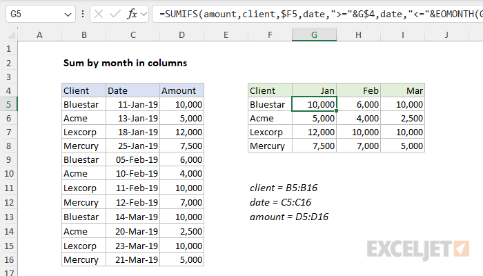
In this example, the values in G4:I4 are actually first-of-month dates, formatted to display only an abbreviated month name. The SUMIFS function is configured to use EOMONTH to create “brackets” for each month that are used to sum the amounts in column D by month and by client. For a full explanation of how this formula works, see this page .
Example - Sequence of months
In Excel 2021 and later, you can use the SEQUENCE function with EOMONTH to create a list of end-of-month dates. In the worksheet below, the start date is in cell B5. The formula in D5 looks like this:
=EOMONTH(B5,SEQUENCE(12))
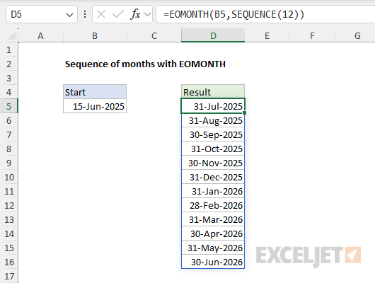
The SEQUENCE function returns an array of 12 numbers like {1;2;3;4;5;6;7;8;9;10;11;12} directly to the EOMONTH function:
=EOMONTH(B5,{1;2;3;4;5;6;7;8;9;10;11;12})
EOMONTH then generates 12 end-of-month dates starting with the month after 15 June 2025. If the date in cell B5 is changed, a new list of dates will be generated. For a more detailed explanation of this idea, see Sequence of months .
Notes
- For months , use a positive number for future dates and a negative number for past dates.
- EOMONTH will return the #VALUE error if the start date is not a valid date.
- If the start date has a fractional time attached, it will be removed.
- If the months argument contains a decimal value, it will be removed.
- To move any date n months into the future or past, see the EDATE function .
- EOMONTH returns a date serial number , which must be formatted as a date .
Explanation
Working from the inside out, we use the DATEDIF function to calculate how many complete years are between the original anniversary date and the “as of” date, where the as of date is any date after the anniversary date:
DATEDIF(B5,C5,"y")
Note: in this case, we are arbitrarily fixing the “as of” date as June 1, 2017 in all examples.
Because we are interested in the next anniversary date, we add 1 to the DATEDIF result, then multiply by 12 to convert to years to months.
Next, the month value goes into the EDATE function, with the original date from column B. The EDATE function rolls the original date forward by the number of months given in the previous step which creates the next upcoming anniversary date.
As of today
To calculate the next anniversary as of today, use the TODAY() function for the “as of” date:
=EDATE(date,(DATEDIF(date,TODAY(),"y")+1)*12)
