Explanation
In this example, the goal is to convert a space-separated sequence of Unicode code points into a readable text string. We can solve this using several Excel functions working together to split, convert, and reconstruct the text. This is the reverse operation of this formula that converts text into Unicode sequence.
The formula explained
The formula processes the Unicode sequence through several steps:
=TEXTJOIN("",,UNICHAR(HEX2DEC(TEXTSPLIT("0061 0070 0070 006C 0065"," "))))
Working from the inside out:
- TEXTSPLIT(“0061 0070 0070 006C 0065”," “) - Splits the sequence string by spaces {“0061”;“0070”;“0070”;“006C”;“0065”}
- HEX2DEC(TEXTSPLIT(…)) - Converts each hexadecimal value to decimal {97;112;112;108;101}
- UNICHAR(HEX2DEC(…)) - Converts each decimal number to its corresponding character {“a”;“p”;“p”;“l”;“e”}
- TEXTJOIN(”",, …) - Joins all characters together without separators
The advantage of this formula over the standard UNICHAR function is that it processes an entire Unicode sequence and returns the complete reconstructed string. This makes it perfect for converting Unicode sequences back to their original text form.
For example, the standard UNICHAR function only converts a single Unicode code point:
=UNICHAR(97) // returns "a"
While this formula processes the complete Unicode sequence:
=TEXTJOIN("",,UNICHAR(HEX2DEC(TEXTSPLIT("0061 0070 0070 006C 0065"," ")))) // returns "apple"
This is especially useful for more complicated Unicode sequences like those that contain special characters or combining characters.
Example #1 - Basic examples
Here are some examples of Unicode sequences and their corresponding text strings:
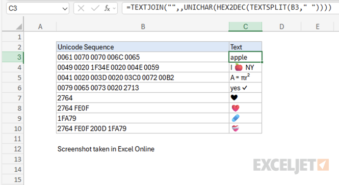
Note: As of this writing in October 2025, emojis in Excel Online (i.e. the web app) appear in color, but emojis in the desktop version of Excel appear in black and white only.
Example #2 - Text with special characters
A practical use-case of this formula is to encode a Unicode sequence that contains special characters back into its corresponding text string.
For example, consider the Unicode sequence “0041 0020 003D 0020 03C0 0072 00B2” that represents the mathematical formula “A = πr²”. Using the formula, we can encode the Unicode sequence to text:
=TEXTJOIN("",,UNICHAR(HEX2DEC(TEXTSPLIT("0041 0020 003D 0020 03C0 0072 00B2"," ")))) // returns "A = πr²"
Breaking down the Unicode sequence the formula processes:
- 0041 - “A” (Latin capital letter A)
- 0020 - " " (space)
- 003D - “=” (equals sign)
- 0020 - " " (space)
- 03C0 - “π” (Greek small letter pi - U+03C0)
- 0072 - “r” (Latin small letter r)
- 00B2 - “²” (superscript two - U+00B2)
This is particularly useful when you have a Unicode sequence from an external source and need to convert it back to readable text.
Example #3 - Text with combining characters
The formula can also handle Unicode sequences that contain combining characters, such as emojis with variation selectors.
For example, the Unicode sequence “2764 FE0F” represents the heart emoji “❤️”. It’s a combination of the basic heart symbol “❤” (U+2764) plus a variation selector (U+FE0F) that tells the system to display it as an emoji rather than a text symbol.
=TEXTJOIN("",,UNICHAR(HEX2DEC(TEXTSPLIT("2764 FE0F"," ")))) // returns "❤️"
For an even more complex example, consider the mending heart emoji “❤️🩹”. It’s a combination of the basic heart symbol “❤” (U+2764) plus a variation selector (U+FE0F) plus a zero-width joiner (U+200D) plus the mending heart symbol “🩹” (U+1FA79). Putting this all together, the Unicode sequence “2764 FE0F 200D 1FA79” represents the mending heart emoji “❤️🩹”.
=TEXTJOIN("",,UNICHAR(HEX2DEC(TEXTSPLIT("2764 FE0F 200D 1FA79"," ")))) // returns "❤️🩹"
For a list of all emojis and their corresponding Unicode sequences, see the Emoji Wizard .
Explanation
At the core, this formula uses the MID function to extract characters starting at the second to last space. The MID function takes 3 arguments: the text to work with, the starting position, and the number of characters to extract.
The text comes from column B, and the number of characters can be any large number that will ensure the last two words are extracted. The challenge is to determine the starting position, which is just after the second to last space. The clever work is done primarily with the SUBSTITUTE function, which has an optional argument called instance number. This feature is used to replace the second to last space in the text with the “@” character, which is then located with the FIND function.
Working from the inside out, the snippet below figures out how many spaces are in the text total, from which 1 is subtracted.
LEN(B5)-LEN(SUBSTITUTE(B5," ",""))-1
In the example shown, there are 5 spaces in the text, so the code above returns 4. This number is fed into the outer SUBSTITUTE function as instance number:
SUBSTITUTE(B5," ","@",4)
This causes SUBSTITUTE to replace the fourth space character with “@”. The choice of @ is arbitrary. You can use any character that will not appear in the original text.
Next, the FIND locates the “@” character in the text:
FIND("@","A stitch in time@saves nine")
The result of FIND is 17, to which 1 is added to get 18. This is the starting position, and goes into the MID function as the second argument. For simplicity, the number of characters to extract is hardcoded as 100. This number is arbitrary and can be adjusted to fit the situation.
Extract last N words from cell
This formula can be generalized to extract the last N words from a cell by replacing the hardcoded 1 in the example with (N-1). In addition, if you are extracting many words, you may want to replace the hardcoded argument in MID, 100, with a larger number. To guarantee you the number is large enough, you could simply use the LEN function as follows:
=MID(B5,FIND("@",SUBSTITUTE(B5," ","@",LEN(B5)-LEN(SUBSTITUTE(B5," ",""))-(N-1)))+1,LEN(B5))
