Formulas are the heart of Excel. They can do everything from basic math to complex data analysis. But sometimes, they don’t work as expected. If you work in Excel a lot, you’ve probably seen many formula errors like #DIV/0, #NAME?, and #N/A. In fact, the more you work with formulas, the more errors you’ll run into :)
Although formulas errors can be scary and frustrating, they are quite useful, because they tell you something is wrong. This is much better than not knowing . The most disastrous Excel problems come from normal-looking worksheets that quietly return incorrect results. Trust me, this is not the kind of problem you want to explain to your boss in a meeting.
Most formula errors are the result of small mistakes, like a typo, the wrong cell reference, or deleting a cell referred to by another formula. When you run into a formula error, don’t panic. Stay calm and methodically investigate until you find the cause. Ask yourself, “What is this error telling me?” Experiment with trial and error. As you gain more experience, you’ll be able to avoid many errors, and more quickly correct errors that do arise.
- About Excel Formula Errors #DIV/0! Error #NAME? Error #N/A Error #NUM! Error #VALUE! Error #REF! Error #NULL! Error #### Error #SPILL! Error #CALC! Error #BLOCKED! Error Circular Reference Errors
- How to find formula errors
- How to fix formula errors
- How to trap errors
- Error-related Functions in Excel
About Excel formula errors
There are 10 different formula errors you are likely to run into at some point as you work with Excel formulas. This section shows examples of each formula error, with information and links on how to correct the error.
#DIV/0! error
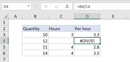
As the name suggests, the #DIV/0! error appears when a formula tries to divide by zero, or by a value equivalent to zero. You may see a #DIV/0! error when data is not yet complete. For example, a cell in the worksheet is blank because data has not been entered, or is not yet available. You also may see the divide by zero error with the AVERAGEIF and AVERAGEIFS functions, when given criteria do not match any cells in the range. For example, in the worksheet below, the DIV error is displayed in cell D4 because C4 is empty. Empty cells are evaluated as zero by Excel, and B4 can’t be divided by zero:
In many cases, empty cells or missing values are unavoidable. You can use the IFERROR function to trap the #DIV/0! and display a more friendly message if you like.
More: How to fix the #DIV/0! error
#NAME? error
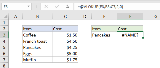
The #NAME? error indicates that Excel does not recognize something. This could be a function name misspelled, a named range that doesn’t exist, or a cell reference entered incorrectly. For example, in the screen below, the VLOOKUP function in F3 is misspelled “VLOKUP”. VLOKUP is not a valid name, so the formula returns #NAME?.
To fix a #NAME? error, you must find the problem, and then correct spelling or syntax. For more details and examples, see this page .
Video: How to use F9 to debug a formula error
#N/A error
The #N/A error appears when something can’t be found. It tells you something is missing or misspelled. This could be a product code not yet available, an employee name misspelled, a color that doesn’t exist, etc. Often, #N/A errors are caused by extra space characters, misspellings, or an incomplete lookup table. The functions most commonly affected by the #N/A error are classic lookup functions, including VLOOKUP, HLOOKUP, LOOKUP, and MATCH. For example, in the screen below, the formula in F3 returns #N/A because “Bacon” is not in the lookup table:
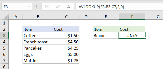
If the value in E3 is changed to an existing value like “Coffee”, “Eggs”, etc. VLOOKUP will work normally and retrieve the item cost.
The best way to prevent #N/A errors is to make sure lookup values and lookup tables are correct and complete. If necessary, you can trap the #N/A error with IFERROR or IFNA and display a more friendly message, or display nothing at all. '
More information: How to fix the #N/A error.
#NUM! error
The #NUM! error occurs when a number is too large or small, or when a calculation is impossible. For example, if you try to calculate the square root of a negative number, you’ll see a #NUM error:
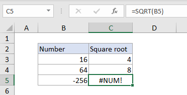
In the screen above the SQRT function is used to calculate the square root numbers in column B. The formula in C5 returns the #NUM! error because the value in B5 is negative, and it is not possible to compute the square root of a negative number.
You might also run into the #NUM error if you reverse start and end dates inside the DATEDIF function . In general, fixing the #NUM! error is a matter of adjusting inputs as required to make a calculation possible again.
More information: How to fix the #NUM! error .
Video: Examples of Excel formula errors
#VALUE! error
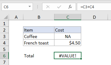
The #VALUE! error appears when a value is not an expected or valid type (i.e. date, time, number, text, etc.) This can happen when a cell is left blank, when a text value is given to a function that expects a numeric value, or when dates are evaluated as text by Excel. For example, in the screen below, cell C3 contains the text “NA”, and the formula in F2 returns the #VALUE! error.
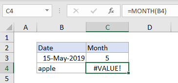
Below, the MONTH function can’t extract a month value from “apple”, since “apple” is not a date:
Note: you may also see a #VALUE! error if you create an array formula and forget to enter the formula with Control + Shift + Enter.
To fix a #VALUE! error, you need to track down the problematic value and supply the right type of value. For more details and examples, see this page .
#REF! error
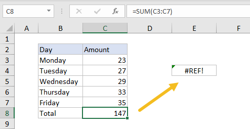
The #REF! error is one of the most common errors you’ll see in Excel formulas. It occurs when a reference becomes invalid. In many cases, this is because sheets, rows, or columns have been removed, or because a formula with relative references has been copied to a new location where references are invalid. For example, in the screen below, the formula in C8 was copied to E4. At this new location, since the range C3:C7 is relative, it becomes invalid and the formula returns #REF!:
#REF! errors can be somewhat tricky to fix because the original cell reference is gone forever. If you delete a row or column and then see #REF! errors, you should undo the action immediately and adjust the formulas first.
More details on #REF! errors.
#NULL! error
The #NULL! error is quite rare in Excel, and is usually the result of a typo where a space character is used instead of a comma (,) or colon (:) between two cell references. For example, in the screen below the formula in F3 returns the #NULL error:
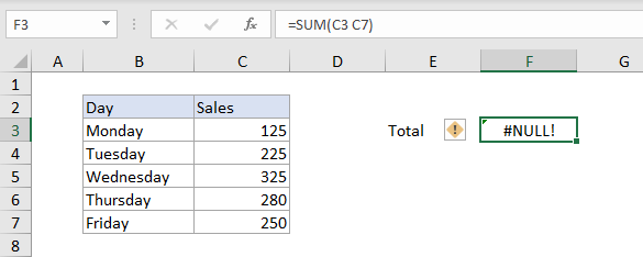
Technically, this is because the space character is the “range intersect” operator and the #NULL! error is reporting that the two ranges (C3 and C7) do not intersect. In most cases, you can correct a NULL error by replacing a space with a comma or colon as needed.
More: How to fix the #NULL! error
#### error
Although technically not an error, you may also see a formula that displays a string of hash characters (###) instead of a normal result. For example, in the screen below, the formula in C3 is adding 5 days to the date in column B:
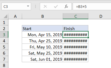
In this case, the hash or pound characters (###) appear because the dates in column C are formatted with a long format and do not fit into the column. To fix this error, just make the column wider.
Note: Excel won’t display negative dates. If a formula returns a negative date value, Excel will display #####.
More: How to fix ##### errors
#SPILL! error
The #SPILL error occurs when a formula outputs a spill range that runs into a cell that already contains data. For example, in the screen below, the UNIQUE function is configured to extract a list of unique names into a spill range starting in D3. Because D5 contains “apple”, the operation is stopped and the formula returns #SPILL!
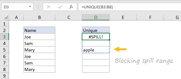
When “apple” is deleted from D5, the formula will work normally, and return “Joe”, “Sam”, and “Mary”.
Details: How to fix #SPILL errors
Video: Spilling and the spill range
#CALC! error
The #CALC error occurs when a formula runs into a calculation error with an array. For example, in the screen below, the FILTER function is set up to filter the source data in B5:D11. However, the formula is asking for all data in the group “apple”, which doesn’t exist:
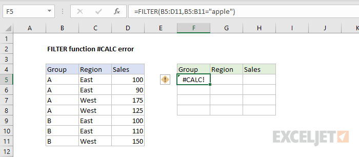
If the formula is adjusted to filter on group “A”, the formula will work normally:
=FILTER(B5:D11,B5:B11="a")
#SPILL! and #CALC! errors are related to " Dynamic Arrays" in Excel 365 and Excel 2021 only.
#BLOCKED! error
The #BLOCKED! error in Excel occurs when certain resources or functions are restricted. The error can occur when a required resource cannot be accessed or by issues such as Excel 4.0 (XLM) macros being disabled. For example, in the worksheet below, the defined name “sheetnames” is based on an older Excel 4.0 macro command called GET.WORKBOOK ( details here ). Because Excel 4.0 macros are disabled in the Trust Centered, Excel returns the #BLOCKED error.
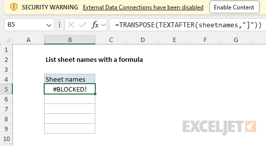
To resolve this error in this particular case, Excel 4.0 macros must be enabled in the Trust Center and the file must be reopened. For a more complete explanation see List sheet names with a formula .
Circular reference errors
A circular reference occurs when a formula refers directly to its own cell, or refers to another cell that depends on the original cell. This creates an infinite loop that cannot be resolved. For example, if cell A1 contains a formula that refers to B1, and B1 contains a formula that refers to A1, this creates a circular reference. Circular reference errors do not appear on the worksheet like other errors in Excel. To find circular references, navigate to Formulas > Error checking > Circular references. For more details see How to fix a circular reference error .
How to find formula errors
There are three basic ways to find formula errors in Excel. The first way is simple observation. Because formula errors are displayed directly on the worksheet they are easy to spot in many worksheets. In larger worksheets or workbooks with many sheets, you can check for errors much faster with Excel’s built-in tools. To select all errors on a given worksheet, you can use Go To Special . To generate a list of all errors in the entire workbook, you can use Find and Replace . Both options are explained below.
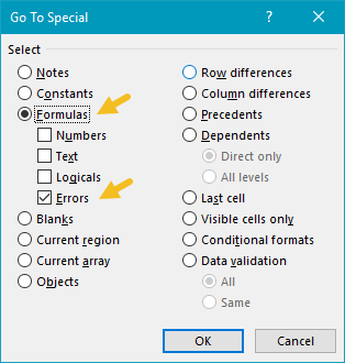
Find errors with Go To Special
You can find all errors at once with Go To Special. Use the keyboard shortcut Control + G, then click the “Special” button. Excel will display the dialog with the options seen below. To select only errors, choose Formulas + Errors, then click “OK”:
After you press OK, Excel will select all errors on the current worksheet. Once selected, you can use the Tab key to move through the selection one cell at a time. If no errors are present, Excel will return the message “No cells were found”.
Note: Go To Special will only find errors on the current worksheet. To find all errors in a workbook, see the next section below.
Find errors with Find and Replace
To find all errors in a workbook across multiple sheets, you can use Find and Replace:
- Open the Find and Replace dialog with the keyboard shortcut Control + F.
- In the “Find what” input area, input the characters “#*!” (without quotation marks).
- Next, select “Workbook” for “Within”, and change “Look in” to “Values”.
- Click the “Find All” button.
- Excel will display a list of matching errors in the workbook as seen below.
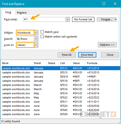
The asterisk (*) is a wildcard in Excel that will match any number of characters, so the idea here is to find values that start with a hash (#) and end with an exclamation point (!). Notice the list of errors contains multiple sheets. To navigate to each error, use the “Find Next” button or click a row in the list.
Notes: (1) The search string “#!” will not find a #N/A error, which does not end with an exclamation point (!). To find #N/A errors, use a more general search string like “#” or a more specific string like “#N/A”. (2) You can also enter individual errors directly. For example, you can enter “#N/A”, “#DIV/0!”, #REF!", etc. to find specific errors.
It is also possible to count errors in a workbook by sheet with a formula.
How to fix formula errors
The basic process for fixing formula errors looks like this:
- Find the errors (see above).
- Identify each error and understand its meaning.
- Trace the error back to its source. If this is difficult, try the trace error feature .
- Figure out what’s causing the error. If needed, break the formula into parts.
- Fix the error at the source or trap the error.
Remember that formula errors often “cascade” through a worksheet, when one error triggers another. As you find and fix the core issue(s), things often come together quickly.
Video: Excel formula error examples
Video: Use F9 to debug a formula
How to trap Errors
Trapping errors is a way of “catching” errors to stop them from appearing in the first place. This makes sense when you know certain errors are likely and you want to stop the errors from appearing on the worksheet. There are two basic approaches:
- Trap the error with IFERROR or ISERROR . With this approach, you are watching for an error, and providing an alternative value when an error is detected. This page shows a VLOOKUP example .
- Prevent calculation until required values are available. In this case, instead of watching for an error, you try to prevent the error from occurring by checking values first. This page shows several examples .
Error-related functions in Excel
Excel provides several error-related functions, each with a different behavior. Click on the links below for more details:
- The ISERR function returns TRUE for any error type except the #N/A error.
- The ISERROR function returns TRUE for any error.
- The ISNA function returns TRUE for #N/A errors only.
- The ERROR.TYPE function returns the numeric code for a given error.
- The IFERROR function traps errors and provides an alternative result.
- The IFNA function traps #N/A errors only and provides an alternative result.
Update: in the current version of Excel you can use the FILTER function to get all matches and the XLOOKUP function to get the last match only. Depending on your needs, FILTER might be a better option than first or last match.
One of the more confusing aspects of lookup functions in Excel is understanding how to get the first or last match in a set of data with more than one match. This is because Excel’s behavior changes depending (1) whether you are performing an exact or approximate match, and (2) whether data is sorted or not.
For example, if we use VLOOKUP to get the price for “green” in the data below, which price will we get?
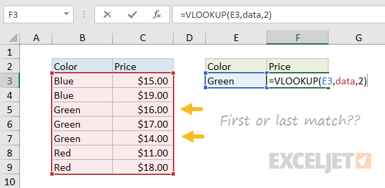
Read on for the answer and more interesting examples.
Notes:
- The examples below use named ranges (as noted in the images) to keep formulas simple.
- Function reference links: VLOOKUP , INDEX , MATCH , and LOOKUP .
Exact match = first
When doing an exact match, you’ll always get the first match, period. It doesn’t matter if data is sorted or not. In the screen below, the lookup value in E5 is “red”. The VLOOKUP function , in exact match mode, returns the price for the first match:
=VLOOKUP(E5,data,2,FALSE)
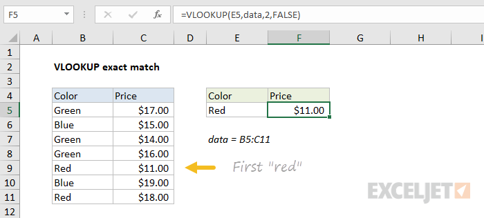
Notice the last argument in VLOOKUP is FALSE to force exact match.
Approximate match = last
If you are doing an approximate match, and data is sorted by lookup value , you’ll get the last match. Why? Because during an approximate match Excel scans through values until a value larger than the lookup value is found, then it “steps back” to the previous value.
In the screen below, VLOOKUP is set to approximate match mode, and colors are sorted. VLOOKUP returns the price for the last “green”:
=VLOOKUP(E5,data,2,TRUE)
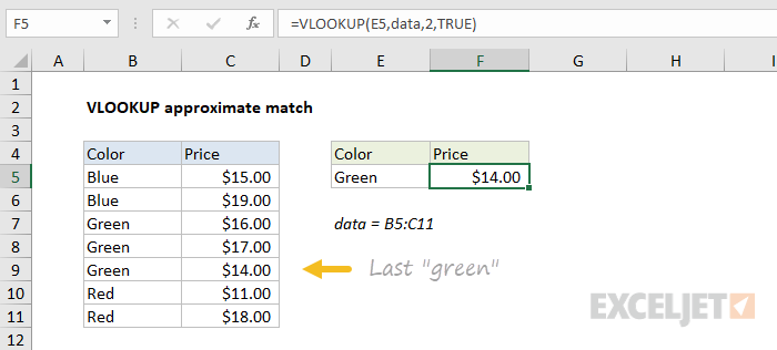
Notice the last argument in VLOOKUP is TRUE for approximate match.
Approximate match + unsorted data = danger
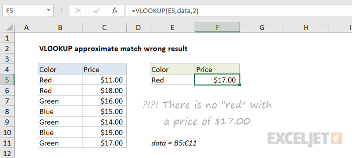
With standard approximate match lookups, data must be sorted by lookup value . With unsorted data, you may see normal-looking results that are totally incorrect. This problem is more likely with VLOOKUP because VLOOKUP defaults to approximate match when no fourth argument is provided.
To illustrate this problem, see the example below. Data is unsorted and VLOOKUP, with no fourth argument provided, defaults to approximate match. Notice there is no “red” with a price of $17.00, yet VLOOKUP happily returns this invalid result:
=VLOOKUP(E5,data,2)
For this reason, I recommend always setting the last argument for VLOOKUP explicitly: TRUE = approximate match, FALSE = exact match. The argument is optional, but providing a value makes you think about it, and provides a visual reminder in the future.
We’ll look at how to overcome the problem of last match and unsorted data below.
“Normal” approximate match
At this point, you may be feeling a little confused and disoriented about the idea that approximate match can return the last match in some cases. If so, don’t worry. Using approximate match to get the last match is not the “normal” case. Typically, you’ll see approximate match used to assign values according to some kind of scale. A classic example is using VLOOKUP in approximate match mode to assign grades, which works beautifully:
=VLOOKUP(E5,key,2,TRUE)
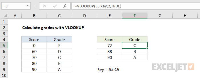
In cases like this, the lookup table deliberately does not include duplicate values, so the whole idea of “last matching value” is irrelevant. More details on this formula here .
The information above is to provide background and context for how matching works in Excel, so that the approaches described below make sense.
Practical applications
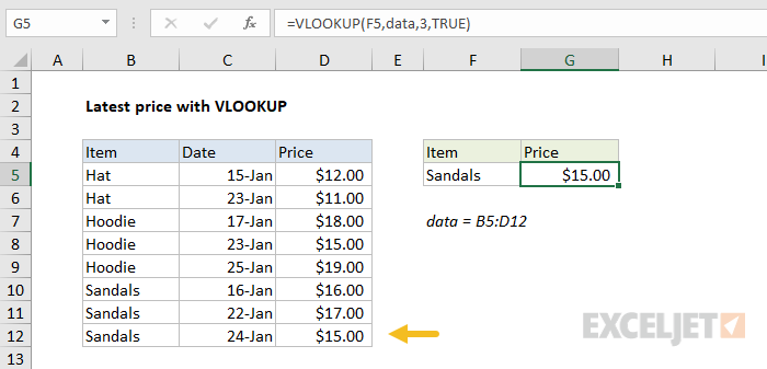
How can we use the behavior described above in a practical situation? Well, one common scenario is looking up the “latest” or “last” entry for an item. For example, below we are using VLOOKUP in approximate match mode to find the latest price for Sandals. Notice data is sorted by item, then by date, so the latest price for a given item appears last:
=VLOOKUP(F5,data,3,TRUE)
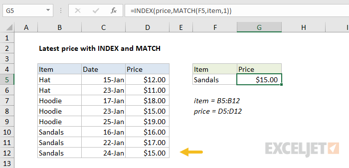
INDEX and MATCH
Other lookup functions can be used this way as well. Below, we are using an equivalent INDEX and MATCH formula find the latest price with the same data. Notice MATCH is configured to approximate match for items sorted in ascending order by setting the third argument to 1:
=INDEX(price,MATCH(F5,item,1))
LOOKUP function
The LOOKUP function can also be used in this case. LOOKUP always performs an approximate match, so it works well in “last match” scenarios. The formula is quite simple:
=LOOKUP(F5,item,price)
Last match with unsorted data
What if you want the last match, but data isn’t sorted by lookup value? In other words, you want to apply criteria to find a match, and you simply want the last item in the data that matches your criteria? This is actually a case where the LOOKUP function shines, because LOOKUP can handle array operations natively, without control + shift + enter. This means we can dynamically build a lookup array to locate the data we want using simple logical expressions.
For example, have a look at the formula below:
=LOOKUP(2,1/(item=F5),price)
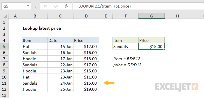
This formula finds the latest price for Sandals in unsorted data.
You may not have seen a formula like this before, so let’s break it down in steps. Working from the inside out, we first apply the criteria with a simple logical expression:
item=F5
This results in an array of TRUE and FALSE values, where TRUE corresponds to items that are “sandals” and FALSE corresponds to all other values:
{FALSE;TRUE;FALSE;TRUE;FALSE;FALSE;TRUE;FALSE}
Next, we divide the number 1 by this array. During division, TRUE becomes 1 and FALSE becomes zero, so you should visualize the operation like this:
1/{0;1;0;1;0;0;1;0}
One divided by one is one, and one divided by zero is #DIV/0, so the result is another array, this one containing only 1s and #DIV/0 errors:
{#DIV/0!;1;#DIV/0!;1;#DIV/0!;#DIV/0!;1;#DIV/0!}
Don’t worry, there is a method to this madness :)
Now, you may have noticed that the lookup value is the number 2. This may seem puzzling. How will LOOKUP ever find the number 2 in an array that contains only 1s and errors? It won’t. We are using 2 as a lookup value to force LOOKUP to scan to the end of the data .
The LOOKUP function will automatically ignore errors, so the only thing left to match are the 1s. It will scan through the 1s looking for a 2 that will never be found. When it reaches the end of the array, it will “step back” to the last valid value – the last 1 – which corresponds to the last match based on criteria provided.
INDEX and MATCH array version
The beauty of the LOOKUP function is it can handle the array operation described above natively in older versions of Excel without requiring you to enter as an array formula with control + shift + enter. However, you can certainly use an array formula if you like. Here is the equivalent INDEX and MATCH formula, which must be entered with control + shift + enter in older versions of Excel:
=INDEX(price,MATCH(2,1/(item=F5),1))
Note: in the current version of Excel , the above formula will just work without special handling. Also, the newer XMATCH function and XLOOKUP function can be directly configured to return the last match.
Last non-blank cell
The approach above turns out to be really useful. For example, by tweaking the logic a bit, we can do things like find the last non-empty cell in a column:
=LOOKUP(2,1/(B:B<>""),B:B)
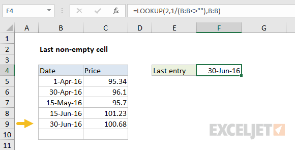
This formula is described in more detail here .
Lookup nth match? All matches?
If you’ve made it this far, you may be wondering how you would find the second or third match, or how you would retrieve all matches? Here are some links for you:
- How to get nth match with VLOOKUP
- How to get nth match with INDEX and MATCH
- How to get all matches INDEX and MATCH
You’ll notice formulas like this get complicated. There are some cool new functions coming to Excel in 2019 that will make these solutions much simpler. Stay tuned. In the meantime, don’t forget that Pivot Tables are a great way to explore data without formulas .
What’s next?
- Formula basics - if you’re just getting started
- 500 formula examples with full explanations
- 101 important Excel functions
- Guide to all Excel functions (work in progress)
- Formula criteria - 50 examples
- Formulas for conditional formatting
