Excel hours
In Excel, dates are just serial numbers, so a single day has a numeric value of 1. This means that 6 hours is one-quarter of a day (0.25), 12 hours is half a day (0.5), 18 hours is three-quarters of a day (0.75), and 24 hours is 1 day. In the same way, 6:00 AM has a numeric value of 0.25, 12:00 PM has a value of 0.5, and 6:00 PM has a value of 0.75. The table below summarizes this relationship:
| Hours | Time | Fraction | Value |
|---|---|---|---|
| 0 | 12:00 AM | 0/24 | 0 |
| 3 | 3:00 AM | 3/24 | 0.125 |
| 6 | 6:00 AM | 6/24 | 0.25 |
| 4 | 4:00 AM | 4/24 | 0.167 |
| 8 | 8:00 AM | 8/24 | 0.333 |
| 12 | 12:00 PM | 12/24 | 0.5 |
| 18 | 6:00 PM | 18/24 | 0.75 |
| 21 | 9:00 PM | 21/24 | 0.875 |
| 24 | 12:00 AM | 24/24 | 1.0* |
- In Excel, midnight (12:00 AM) has a dual nature: it has a value of 0 when it represents the start of a day, but it can be 1 inside a calculation that completes a full 24-hour cycle. In other words, as we approach midnight, the value of time approaches 1. But as we cross from one day to another, the 1 is added to the date, and time begins again at zero.
Formatting time
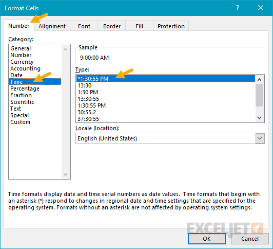
Time is displayed in Excel using a number format for time. To apply one of Excel’s built-in number formats for time, follow this process:
- Select the cells you want to format as time.
- Open the Format Cells dialog ( keyboard shortcut : Control + 1)
- Navigate to Number > Time
- Select the Time format you want to apply and click OK.
Duration over 24 hours
To calculate and display time durations over 24 hours, you’ll want to use a custom time format like [h]:mm. Otherwise, the duration will appear to “reset” every 24 hours when the date is incremented by 1, in the same way that a clock “resets” each day. More on custom number formats here .
Convert Excel time to decimal hours
To convert fractional time to decimal hours, just multiply by 24. For example, 0.5* 24 = 12 hours, 0.25* 24 = 6 hours, etc. For more details, see Convert Excel time to decimal value .
An expanding reference (or expanding range) in Excel defines a range that expands as a formula is copied down or across cells. This is done by “mixing” absolute and relative references – making the first cell an absolute reference and the last cell a relative reference .
Example
In the example shown the formula in D4 is:
=SUM($C$4:C4)
As this formula is copied down column D, it changes as follows:
=SUM($C$4:C4) // D4
=SUM($C$4:C5) // D5
=SUM($C$4:C6) // D6
At each new row, the range is expanded to include one new row. As a result, the SUM function calculates an accurate running total.
