Explanation
In this example, the goal is to extract a date in a format like mm/dd/yy from a text string with a formula. The position of the date is not known, so the date must be located as a first step. This article explains two ways to solve this challenge:
- A “classic” formula based on the SEARCH function and the MID function that will work in any version of Excel.
- A modern formula based on the REGEXEXTRACT function, which is only available in the Beta channel of Excel 365.
Classic formula
In the worksheet shown, we are using a “classic” formula to extract dates from the text strings in column B. The formula in cell D5 looks like this:
=MID(B5,SEARCH("??/??/??",B5),8)+0
At a high level, this formula uses the SEARCH function to locate the date and the MID function to extract the date. MID is designed to extract a given number of characters from the middle of a text string. SEARCH will return the position of a matching value as a number. Working from the inside out, SEARCH is configured like this:
SEARCH("??/??/??",B5)
Here, the find_text is given as “??/??/??”, and the within_text is provided as B5. The SEARCH supports wildcards, and the “?” character means any single character . The pattern “??/??/??” means: any two characters followed by a forward slash “/”, followed by any two characters followed by a forward slash “/”, followed by any two characters .
The text in cell B5 is 57 characters long, and the date begins at character 37. The SEARCH function finds the date pattern and returns 37 as a result. This result lands inside the MID function as the start_num . Simplifying, we now have:
=MID(B5,37,8)+0
Inside the MID function, the text comes from cell B5, the start_num is 37, and num_chars is set to 8. We use 8 because a date in the format “mm/dd/yy” is eight characters. With this configuration, MID extracts 8 characters beginning at character 37, and we now have the date isolated, still in text format:
="06/15/24"+0
As a final step, we add zero. This is a simple hack to get a valid date from a text string. The math operation forces Excel’s formula engine to try and convert the text “06/15/24” into a number. In this case, Excel recognizes that “06/15/24” as a date and performs the conversion. It then returns the serial number 45458, which is June 15, 2024, in Excel’s date system :
=45458+0
Adding zero has no effect on the number, so the final result is 45458. The last step is to format the result using the date format “d-mmm-yyyy” which causes Excel to display the dates in column D as they appear. We can apply this formatting because we have converted text value into a valid Excel date. This format can be adjusted to display dates as desired.
Why add zero? When extracting a date from a text string using a formula, the result is initially returned as text. By adding zero (+0), we force Excel to interpret the text as a number, which automatically converts the text string into a valid Excel date. This step is important because Excel stores dates as serial numbers. Once converted, the date can be formatted and used in calculations like any other date value. Without this step, Excel would not recognize the text as a date.
Although this formula is fairly simple, it is not especially robust. For example, it will match the non-date “AA/BB/CC” and even “AAAA/BB/CCCC”. It will also fail on dates in “mm/dd/yyyy” format since only the first two year digits of the year will be used, resulting in an incorrect year. If all dates use a 4-digit year, you can use the modified formula below:
=MID(B5,SEARCH("??/??/????",B5),10)+0
See below for a more robust formula based on regex.
Notes: (1) If you only want a text value (not an actual date), omit adding a zero. (2) This formula works because the SEARCH function supports wildcards, unlike the FIND function .
A modern formula based on regex
In the latest version of Excel, which offers the REGEXEXTRACT function , we can build a more robust formula because regex patterns are much more specific than Excel’s primitive wildcards. In the worksheet below, we are using REGEXEXTRACT to extract dates with a formula like this:
=REGEXEXTRACT(B5,"\b\d{1,2}/\d{1,2}/\d{2,4}\b")+0
Inside REGEXEXTRACT, the text is given as B5. The regex pattern looks like this:
"\b\d{1,2}/\d{1,2}/\d{2,4}\b"
Regular expressions (regex) are a language used to match and extract text patterns. Briefly, this is how the pattern works:
- \b: Matches a word boundary
- \d{1,2}: Matches one or two digits for the month
- /: Matches the forward slash separator
- \d{1,2}: Matches one or two digits for the day
- /: Matches the second forward slash separator
- \d{2,4}: Matches 2-4 digits for the year
- \b: Matches another word boundary
You can see how the formula works in the worksheet below:
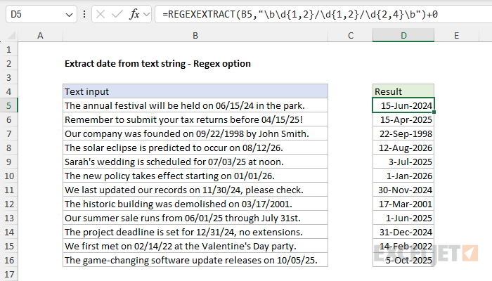
Notice we are now matching 4-digit years on rows 7 and 12, in addition to the other 2-digit years. Compared to the MID + SEARCH formula above, this formula does a better job of matching dates. It is more flexible in some ways but more restrictive in others. For example, it will match dates like “1/1/23”, “01/01/23”, and “5/25/2023”, but it won’t match a text string like “AA/BB/CC” or “1234/12/1234”. However, note that the pattern does not check that the month is between 1-12 or that the day is valid for the given month. It also doesn’t validate the year in any way. It would, for example, allow a 3-digit year, which Excel won’t interpret correctly. Since this is regex, we can easily make the pattern more specific. The revised formula below will only allow a 2-digit year OR a 4-digit year:
=REGEXEXTRACT(B5,"\b\d{1,2}/\d{1,2}/(\d{2}|\d{4})\b")+0
In regex, there is always a way to tighten up edge cases at the cost of more complexity. However, even the initial regex formula above is much better than the traditional SEARCH + MID at preventing false matches. REGEXEXTRACT is a huge upgrade to Excel’s tools for matching and extracting text.
Explanation
In this example, the goal is to extract the time portion of a date that contains time (also called a “datetime”). Since dates in Excel are serial numbers and times are fractional values of a day, the task is to extract the decimal portion of the serial number. This is easy to do with the MOD function, and other methods mentioned below. Note that if you are comparing extracted times to other time values, there is a subtle floating point precision issue you should be aware of.
- How Excel handles dates and times
- Using MOD to extract time
- Other methods to extract time
- Floating point precision issue
- Workaround: use TIME or ROUND
How Excel handles dates and times
Excel handles dates and times using a system in which dates are serial numbers and times are fractional values of a day. For example, June 1, 2000 12:00 PM is represented in Excel as the number 36678.5, where 36678 is the date (June 1, 2000) and .5 is the time (12:00 PM). Since 12:00 PM is exactly halfway through a day, Excel represents it as 0.5. Likewise, 6:00 AM is 0.25 (one quarter of a day) and 6:00 PM is 0.75 (three quarters of a day). In other words, the time value in a “datetime” is the decimal portion of the number.
Using MOD to extract time
The MOD function returns the remainder from division. The first argument is the number and the second is the divisor. Here are a few examples:
=MOD(5,2) // returns 1
=MOD(7,5) // returns 2
If you use MOD with a divisor of 1, the result will be the decimal part of the number, if any, because every whole number can be evenly divided by itself. For example:
=MOD(3.5,1) // returns 0.5
=MOD(3.125,1) // returns 0.125
In short, =MOD(number,1) returns just the fractional part of a number, discarding the integer portion, so it’s a convenient way to extract time from a date.
If you use this formula to strip the time from a date + time, you’ll need to apply a suitable number format to display as time.
Other methods to extract time
What’s nice about MOD is that it’s a simple one-function solution. However, there are other ways to extract time from a datetime. The most common alternatives subtract the integer (date) portion from the original value using the INT function or the TRUNC function :
=B5-INT(B5)
=B5-TRUNC(B5)
Both formulas work the same way: they calculate the date portion and subtract it from the datetime, leaving just the time. Another option is to rebuild the time from its components using TIME , HOUR , MINUTE , and SECOND :
=TIME(HOUR(B5),MINUTE(B5),SECOND(B5))
This approach extracts each time component as an integer, then reassembles them into a time value. This is a more verbose formula, but it has the advantage of avoiding the floating-point precision issue described below.
Floating point precision issue
The MOD formula works well for displaying extracted times, but there’s a subtle gotcha you should know about. Because of the way computers handle decimal numbers (known as floating point arithmetic ), the result from MOD may not be exactly equal to the same time created with the TIME function . This can cause problems when comparing extracted times.
For example, say you have a datetime like October 20, 2024, 4:00 PM in cell A1. If you extract the time with MOD and compare it to 4:00 PM created with TIME, you might expect them to be equal:
=MOD(A1,1)=TIME(16,0,0) // may return FALSE!
The result may be FALSE because MOD returns something like 0.6666666666642413 instead of 0.666666666666667 (the value TIME returns for 4:00 PM). The difference is tiny (invisible when formatted as time) but enough to break equality checks. You can see examples of these very slightly different values for 1:00 PM and 4:00 PM in cells E15 and E16, respectively:

This issue isn’t specific to MOD. Any formula that uses subtraction to isolate the time portion will have the same problem, including formulas based on INT, TRUNC, and DATE :
=A1-INT(A1) // same issue
=A1-TRUNC(A1) // same issue
=A1-DATE(YEAR(A1),MONTH(A1),DAY(A1)) // same issue
Workaround: use TIME or ROUND
If you need to compare extracted times to other time values, here are two reliable solutions. The first option is to rebuild the time with TIME. The formula extracts the hour, minute, and second with HOUR, MINUTE, and SECOND, then rebuilds the time value using TIME:
=TIME(HOUR(B5),MINUTE(B5),SECOND(B5))
Because TIME builds the time from scratch using integer values, it avoids the precision issue entirely.
Another good option is to round before comparing values with the ROUND function . Rounding to about 10 decimal places is enough:
=ROUND(MOD(B5,1),10)=ROUND(TIME(16,0,0),10) // reliable comparison
Either approach will give you consistent results when comparing times.
