Explanation
In this example, the goal is to extract the numbers from a set of property listings which describe the number of bedrooms and bathrooms, the size of the house in sq. ft., and the size of the lot in acres. Traditionally, this kind of problem has been quite difficult in Excel because each number must be extracted with a separate, carefully configured formula ( example ). However, in the latest version of Excel, new functions like TEXTSPLIT, TOROW, and DROP make the process much easier.
The approach
The overall approach in the worksheet shown above is to split the text in column B into separate words, remove all non-numeric words with a clever hack, and remove the first number, which represents the street number. The formula in cell C5, copied down, looks like this:
=DROP(TOROW(TEXTSPLIT(B5," ")+0,2),,1)
Working from the inside out, the first step is to split the text string into separate words.
Splitting text into words
To split the text strings in column B into separate words, we use the TEXTSPLIT function . TEXTSPLIT is a flexible function that can be configured with up to six arguments, but in this case, we need just two: text and column delimiter:
TEXTSPLIT(B5," ") // split text into words
For text , we provide cell B5. For col_delimiter, we provide a single space (" “). With these inputs, TEXTSPLIT splits the text at each space and returns an array like this:
{"1025","Maple","St,","4","beds","3","baths,","3200","sq.","ft.","on",".35","acre"}
Note that all values at this point are text strings, which Excel encloses in double quotes (”").
Removing the non-numeric values
The next step in the process is to remove the non-numeric values. At first glance, this is a puzzle, because all the values in the array are text, including the numbers. This is one of those cases where the easiest solution is a hack that depends on knowing how the Excel formula engine works. Briefly, Excel tries to convert a text string to a number when it is involved in a math operation. For example, if we add 1 to a true number and a number that is text, it works in both cases:
=100+1 // returns 101
="100"+1 // returns 101
This happens because Excel silently converts the text “100” into the number 100 and then proceeds with the addition. However, if we try to add a number to a text string that can’t be converted to a number, the operation fails with a #VALUE! error:
="apple"+1 // returns #VALUE!
It turns out that we can use this behavior in this problem to easily remove the non-numeric values. First, we add zero to the result from TEXTSPLIT:
TEXTSPLIT(B5," ")+0
As explained above, Excel will try to convert the text values returned by TEXTSPLIT into numbers. The result is an array like this:
{1025,#VALUE!,#VALUE!,4,#VALUE!,3,#VALUE!,3200,#VALUE!,#VALUE!,#VALUE!,0.35,#VALUE!}
Notice #VALUE! errors have replaced the non-numeric text values, while the numbers have survived the operation and are now true numeric values. In other words, we have forced all text values to errors and converted text to numbers at the same time. Next, we need to discard the errors. While we could use the FILTER function for this job, a simpler option is to use the TOROW function like this:
TOROW(TEXTSPLIT(B5," ")+0,2)
The purpose of TOROW is to transform an array into a single row. In this case, we already have a row, so we only use the TOROW function to remove errors, by setting the ignore argument to 2. The result from this operation is a much cleaner array like this:
{1025,4,3,3200,0.35}
With ignore set to 2, TOROW removes the errors and leaves the numbers. Pretty cool, huh?
Removing the street number
The last step in this problem is to remove the first number from the final result, which is a street number, and a characteristic of the property itself. We can do this with the DROP function , which is designed to remove rows or columns from an array. In this case, since we have already split the text into separate columns, we want to remove the first column. We can do that by providing the number 1 for the columns argument:
=DROP({1025,4,3,3200,0.35},,1)
Notice the rows argument is left empty. The final result is an array with four numbers like this:
{4,3,3200,0.35}
This array spills into the range C5:F5. As the formula is copied down, the formula extracts the same information from each property as shown.
With the FILTER function
Just for the record, here is what a formula based on FILTER would look like, instead of TOCOL:
=DROP(FILTER(TEXTSPLIT(B5," ")+0,ISNUMBER(TEXTSPLIT(B5," ")+0),2),,1)
The basic mechanics are the same. TEXTSPLIT creates an array of values, and adding zero forces the text values to errors, leaving numbers. The FILTER function then removes the errors by testing for numbers with the ISNUMBER function . However, because of the structure of FILTER, we need to repeat the TEXTSPLIT operation twice. The TOCOL solution avoids this redundancy, resulting in a compact, elegant formula.
Explanation
In this example, the goal is to use a single formula to extract high-value projects and list them in a simple table. We also want to remove unnecessary columns to create a clean, uncluttered view. The solutions explained below are based on a combination of several functions in Excel, including FILTER, SORT, TAKE, and CHOOSECOLS. This is a useful technique for creating a simple dashboard report with a dynamic set of data. The beauty of this approach is that the original data remains untouched and can be easily updated at any time. In addition, the source data can be located on a different worksheet. You can use this same idea in many ways, for example:
- Create a summary of top-selling products for the current month.
- Create a sales performance dashboard to highlight top-performing sales representatives.
- Create a list of the largest outstanding invoices over 30 days due.
- Create a leaderboard to display the most productive groups or employees.
The article below describes two methods to solve this challenge. The first method uses the FILTER function to extract data of interest. This is the best approach when the logic needed to select important data is more complex. The second approach uses the TAKE function to grab the most important records after sorting. This is an elegant way to build a summary of the “Top n projects”, “Top 5 outstanding payments”, etc.
Method 1: FILTER, SORT, and CHOOSECOLS
The first method to filter and exclude columns is based on the FILTER, SORT, and CHOOSECOLS functions. This is the solution shown in the workbook above, where the formula in cell F4 is:
=CHOOSECOLS(SORT(FILTER(B9:G20,E9:E20>90000),4,-1),1,4)
Working from the inside out, the FILTER function is configured to extract projects with a value over 90,000 like this:
=FILTER(B9:G20,E9:E20>90000)
- array - provided as all data in B9:G20.
- include - provided as the logical expression E9:E20>90000.
- if_empty - Not provided.
The advantage of using FILTER is that we can configure the logic used to select data to apply even complex multiple criteria . This is a more powerful way to isolate important information compared to sorting only.
In the next step, FILTER returns a filtered array of data to the SORT function, which is configured to sort the data by value in descending order:
SORT(FILTER(...),4,-1)
- array - delivered by FILTER.
- sort_index - provided as 4 to sort by Value.
- sort_order - provided as -1 to sort in descending order.
The last step is to remove any columns we don’t want in the final output, which is done with the CHOOSECOLS function :
=CHOOSECOLS(SORT(...),1,4)
- array - provided by SORT.
- col_num1 - provided as 1 to extract Project.
- col_num2 - provided as 4 to extract Value.
CHOOSECOLS is a simple function designed to select specific columns from a set of data by index number. In this case, we want to retain column 1 (Project) and column 4 (Value) so we provide 1 and 4.
Note: We could sort the data before filtering with the same result. However, using FILTER first is more efficient since we are only sorting records that meet our criteria.
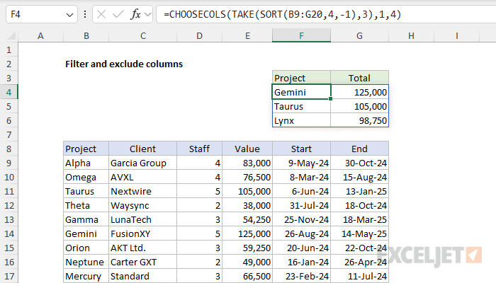
Method 2: SORT, TAKE, and CHOOSECOLS
Another way to filter and exclude columns is to use the TAKE function instead of the FILTER function. This approach makes sense when sorting alone is enough to “surface” the most important data. Once we have data sorted in the preferred order, we use the TAKE function to collect the number of rows desired. For example, to list the top 3 projects by value, we can use a formula like this:
=CHOOSECOLS(TAKE(SORT(B9:G20,4,-1),3),1,4)
You can see the result in the worksheet below:
In the first step, the SORT function is configured to sort all projects by value in descending order like this:
SORT(B9:G20,4,-1)
- array - provided as B9:G20 (12 rows)
- sort_index - provided as 4 to sort by Value.
- sort_order - provided as -1 to sort in descending order.
In the next step, SORT returns a sorted array of data to the TAKE function , which is configured to extract the first 3 rows:
TAKE(SORT(...),3)
- array - delivered by SORT.
- rows - provided as 3.
The last step is to remove any columns we don’t want in the final output, which is done with the CHOOSECOLS function as before. Because we want to retain column 1 (Project) and column 4 (Value), we provide 1 and 4:
=CHOOSECOLS(TAKE(...),1,4)
- array - provided by TAKE.
- col_num1 - provided as 1 to extract Project.
- col_num2 - provided as 4 to extract Value.
Conclusion
In this article, we looked at two ways to filter and exclude columns from a dataset in Excel using a combination of FILTER, SORT, TAKE, and CHOOSECOLS functions. These techniques are useful for creating simple, dynamic summaries that update automatically as the source data changes.
- Use the FILTER method when you need to apply more complex logic to select data. FILTER is an excellent tool for identifying and isolating important information based on multiple criteria.
- Use the TAKE method when sorting alone is enough to surface data of interest. This method is ideal for creating summaries like “Top 3 projects” or “Top 5 outstanding payments.” TAKE is also a good choice when you want to limit the number of records displayed.
In the example shown, both methods work well. But note that if more rows were returned by FILTER, more rows would appear in the final result, so we would need to make room for this additional information.
Wait, what about Pivot Tables?
Yes, you can definitely solve this challenge with a Pivot Table as well. In fact, the workbook attached to this article has a working Pivot Table on Sheet3. Until a couple of years ago, Pivot Tables were the best way to solve this challenge. These days, the main reason to use a Pivot Table instead of a formula is that you are working in an older version of Excel without modern functions like FILTER, SORT, TAKE, and CHOOSECOLS. The main disadvantage of a Pivot Table is that it won’t refresh automatically when data changes; you will need to refresh manually. In contrast, a formula-based table will recalculate when any data changes. For more information on Pivot Tables, see:
- Excel Pivot Tables (overview)
- Why Pivot Tables (video)
Note: The video above is now somewhat dated because new functions have made it much easier to summarize data in Excel. In addition, two brand new functions, GROUPBY and PIVOTBY , directly mimic Pivot Table functionality .
