Explanation
A common situation in Excel is to use the SORT function to sort results returned by the FILTER function . However, a formula based on the FILTER and SORT may return an error when no data is returned. In this example, the goal is to create a formula based on FILTER and SORT that will not return an error when the FILTER function returns no data.
Problem
The formula below returns a #CALC! error because there are no rows in the data with dates between April 1 and April 30:
=SORT(FILTER(data,(data[Date]>=F4)*(data[Date]<=F5)),2)
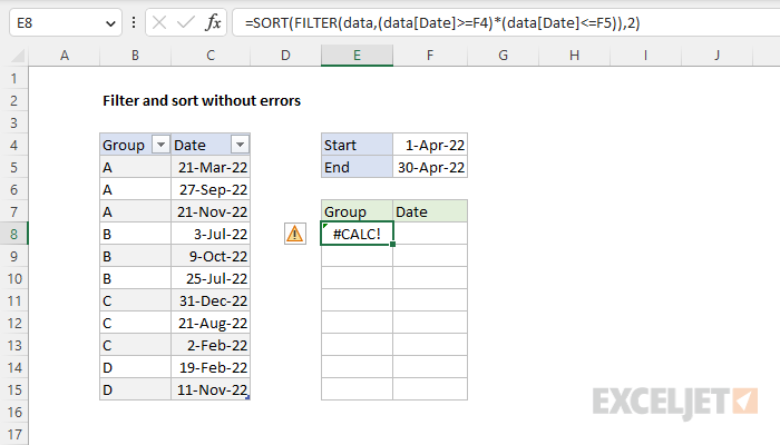
This happens because when FILTER returns no data, it returns a #CALC error by default and this error “bubbles up” to SORT. You might try to handle this problem by providing a value for the if_empty argument in FILTER like this:
=SORT(FILTER(data,(data[Date]>=F4)*(data[Date]<=F5),"No data"),2)
However, this causes the SORT function to return a #VALUE! error, because SORT is configured to sort by column index 2, and there is no second column when the text string “No data” is returned by FILTER:
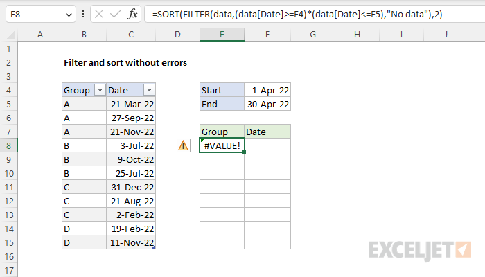
In other words, when FILTER returns “No data” as a result, the configuration for SORT no longer works.
Solution
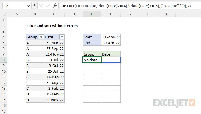
One solution to the problem described above is to provide an array constant like this to FILTER as the if_empty argument:
{"No data",""}) // array constant
The array constant is set up to be a horizontal array by using a comma instead of a semi-colon. The first cell contains “No data” and the second cell is empty. The entire formula looks like this:
=SORT(FILTER(data,(data[Date]>=F4)*(data[Date]<=F5),{"No data",""}),2)
Now when FILTER returns no data, it returns the message “No data” as a two column array constant, and the SORT function harmlessly “sorts” the array constant by the second column and returns it unchanged to cell E8 where it spills into the range E8:F8:
Array constant size
In general, you should adjust the array constant to match the number of columns in the data supplied to FILTER. For example, if the data had 4 columns, you could use an array constant with 4 values like this:
{"No data","","",""} // 4 values
This allows the SORT function to be configured to sort by any column without an error. Also note you can supply whatever values you like in the array constant; empty strings are not required.
Explanation
The goal is to filter the horizontal data in the range C4:L6 to extract members of the group “fox” and display results with data transposed to a vertical format. For convenience and readability, we have two named ranges to work with: data (C4:L6) and group (C5:L5).
The FILTER function can be used to extract data arranged vertically (in rows) or horizontally (in columns). FILTER will return the matching data in the same orientation. The formula in B5 is:
=TRANSPOSE(FILTER(data,group="fox"))
Working from the inside out, the include argument for FILTER is a logical expression:
group="fox" // test for "fox"
When the logical expression is evaluated, it returns an array of 10 TRUE and FALSE values:
{TRUE,FALSE,TRUE,FALSE,FALSE,TRUE,TRUE,TRUE,TRUE,FALSE}
Note: the commas (,) in this array indicate columns. Semicolons (;) would indicate rows.
The array contains one value per record in the data, and each TRUE corresponds to a column where the group is “fox”. This array is returned directly to FILTER as the include argument, where it does the actual filtering:
FILTER(data,{TRUE,FALSE,TRUE,FALSE,FALSE,TRUE,TRUE,TRUE,TRUE,FALSE})
Only data in columns that correspond to TRUE make it through the filter, so the result is data for the six people in the “fox” group. FILTER returns this data in the original horizontal structure. Because we want to display results from FILTER in a vertical format, the TRANSPOSE function is wrapped around the FILTER function:
=TRANSPOSE(FILTER(data,group="fox"))
The TRANSPOSE function transposes the data and returns a vertical array as a final result in cell B10. Because FILTER is a dynamic array function , the results spill into the range B10:D15. If data in data (C4:L6) changes, the result from FILTER is automatically updated.
Dynamic Array Formulas are available in Office 365 only.
