Filter By Column, Sort By Row

Explanation

Note: FILTER is a new dynamic array function in Excel 365 . In other versions of Excel, there are alternatives , but they are more complex.

In this example, the goal is to filter the data shown in B5:G15 by year, then sort the results in descending order. In addition, the result should include the Group column, sorted in the same way. The problem breaks down into two main steps:

1. Filter to select the Group and matching Year column
2. Sort the result in descending order by year values

Filter by column

To filter the data to select the Group column and data for the matching year, we use the FILTER function . Typically FILTER is used to filter data vertically, selecting rows that match provided conditions. However, FILTER can also select data horizontally. The key is to provide logic for the include argument that will return a horizontal array with the same number of columns as the source data. For example, to return data for the year 2017, we can use a formula like this:

=FILTER(B5:G15,B4:G4=2017)

The logical expression:

=B4:G4=2017

returns a one-row horizontal array with 5 columns:

{FALSE,FALSE,TRUE,FALSE,FALSE,FALSE}

When provided to FILTER as the include argument , FILTER returns the values for 2017 only:

FILTER(B5:G15,{FALSE,FALSE,TRUE,FALSE,FALSE,FALSE}) // 2017 only

To add in the Group column, we extend the logic using Boolean logic , a technique for working with TRUE and FALSE values as 1s and 0s. In Boolean algebra, multiplication corresponds to AND logic, and addition corresponds to OR logic . In this case, we want FILTER to return the Group column and the matching year column. This means we need OR logic - i.e. column = “group” OR column = [year].

Using addition for OR logic, we can construct an expression like this:

=(B4:G4="group")+(B4:G4=2017)

This results in two arrays with TRUE and FALSE values, joined by addition:

{TRUE,FALSE,FALSE,FALSE,FALSE,FALSE} +
{FALSE,FALSE,TRUE,FALSE,FALSE,FALSE}

The math operation of addition coerces the TRUE and FALSE to numbers, and the result is a single array of 1s and 0s:

{1,0,1,0,0,0}

Notice the first and third columns are 1, while the other columns are 0. When this array is provided to FILTER as the include argument, FILTER returns columns 1 and 3 from the data.

Sort by row

Because the FILTER function is nested inside the SORT function . FILTER returns the two matching columns explained above directly to SORT:

=SORT(filter_result,2,-1)

We want to sort these columns by values in the year column (2017) in descending order, so sort_index is provided as 2, and sort_order is given as -1. With these inputs, the SORT function returns the sorted as shown in the example. Notice that Group E appears first since 27% is the highest value in 2017.

When the year in J4 is changed, FILTER selects new columns, and the SORT function sorts the new data in the same way.

Dropdown menu for year

To make the year dropdown menu, you can apply a simple data validation rule to cell J4. The allowed values are based on the existing years in C4:G4, with In-cell dropdown selected:

Once data validation is in place, a dropdown menu with the years 2016-2020 will appear. If you are new to data validation, see our Data Validation Guide .

Explanation

This example shows how to filter dates using Excel’s FILTER function. Several common date-based filtering patterns are shown below, including filtering by month, filtering by a specific date, and filtering by month and year.

Filter by month

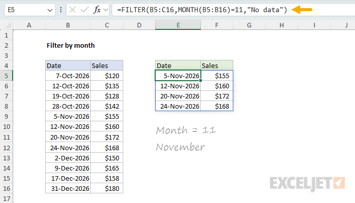
In the worksheet below, the goal is to filter the data to include only rows where the date falls in November. The formula in cell E5 is:

=FILTER(B5:C16,MONTH(B5:B16)=11,"No data")

Note that the month is hardcoded as the number 11. The result returned by FILTER includes only rows where the date falls in November:

This formula relies on the FILTER function to retrieve data based on a logical test created with the MONTH function . The array argument is B5:C16, which contains the full set of data without headers. The include argument is constructed with the MONTH function:

MONTH(B5:B16)=11

Here, MONTH receives the range B5:B16. Since the range contains 12 cells, MONTH returns an array with 12 results representing each date’s month number:

{10;10;10;10;11;11;11;11;12;12;12;12}

Each result is then compared to 11 (November), and this operation creates an array of 12 TRUE and FALSE values, which is delivered to the FILTER function as the include argument:

{FALSE;FALSE;FALSE;FALSE;TRUE;TRUE;TRUE;TRUE;FALSE;FALSE;FALSE;FALSE}

FILTER uses this array to select specific rows. Only rows where the result is TRUE make it into the final output. The if_empty argument is set to “No data” in case no matching data is found.

Filter by specific date

To filter by a specific date, use the DATE function to construct the date value for comparison. You can see how this works in the worksheet below, where the formula in E5 is:

=FILTER(B5:C16,B5:B16=DATE(2026,11,24),"No data")

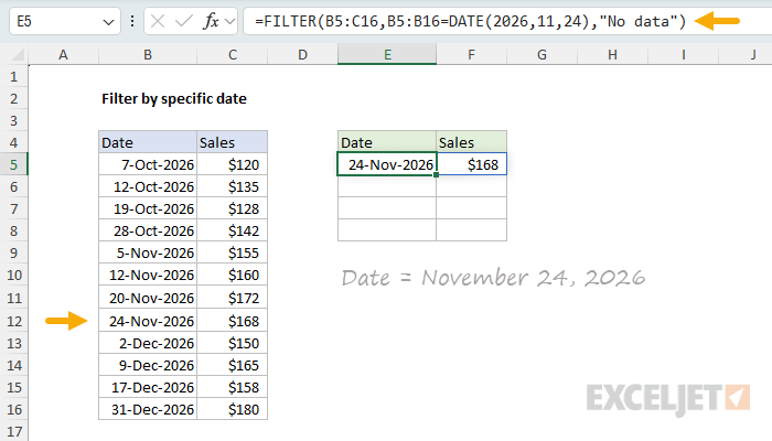
The DATE function creates a proper Excel date from the year (2026), month (11), and day (24). This is compared against each date in the range B5:B16. Only the row matching November 24, 2026 is returned.

Filter by month and year

To filter by both month and year, you can construct a formula using boolean logic that combines the YEAR function and MONTH function :

=FILTER(B5:C16,(YEAR(B5:B16)=2026)*(MONTH(B5:B16)=12),"No results")

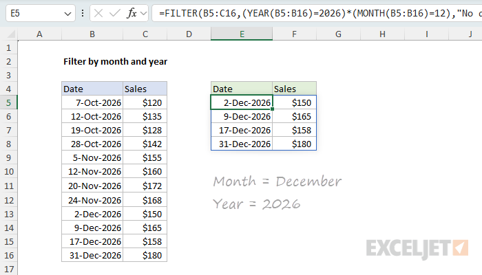
The multiplication operator (*) acts as an AND condition—both the year must equal 2026 and the month must equal 12 (December) for a row to be included. This returns all four December 2026 dates from the source data.

Although the values for month and year are hardcoded in this example (the year is 2026 and the month is 12), these values can easily be replaced with cell references to make the formula more flexible.

Summary

The FILTER function can extract data by date in different ways using Excel’s date functions:

• Use MONTH, YEAR, DAY, or WEEKDAY to extract date components
• Compare extracted values to target values to create a Boolean array
• Combine multiple criteria with multiplication (AND logic)
• Use cell references instead of hardcoded values for flexibility

For filtering between two dates, see Filter data between dates .