Explanation
The FILTER function is designed to extract data that matches one or more criteria. In this case, we want to apply criteria that requires all three columns in the source data (Name, Group, and Room) to have data. In other words, if a row is missing any of these values, we want to exclude that row from output.
To do this, we use three boolean expressions operating on arrays. The first expression tests for blank names:
B5:B15<>"" // check names
The not operator (<>) with an empty string ("") translates to “not empty”. For each cell in the range B5:B15, the result will be either TRUE or FALSE, where TRUE means “not empty” and FALSE means “empty”. Because there are 11 cells in the range, we get 11 results in an array like this:
{TRUE;FALSE;TRUE;TRUE;TRUE;TRUE;TRUE;TRUE;TRUE;FALSE;TRUE}
The second expression tests for blank groups:
C5:C15<>"" // check groups
Again, we are checking 11 cells, so we get 11 results:
{TRUE;TRUE;TRUE;FALSE;TRUE;TRUE;TRUE;TRUE;FALSE;FALSE;TRUE}
Finally, we check for blank room numbers:
D5:D15<>"" // check groups
which produces:
{TRUE;TRUE;TRUE;TRUE;TRUE;TRUE;TRUE;FALSE;TRUE;FALSE;TRUE}
When the arrays that result from the three expressions above are multiplied together, the math operation coerces the TRUE and FALSE values to 1s and 0s. We use multiplication in this case, because we want to enforce “AND” logic: expression1 AND expression2 AND expression3. In other words, all three expressions must return TRUE in a given row.
Following the rules of boolean logic, the final result is an array like this:
{1;0;1;0;1;1;1;0;0;0;1}
This array is delivered directly to the FILTER function as the include argument. FILTER only includes the 6 rows that correspond to 1s in the final output.
Explanation
Note: FILTER is a new dynamic array function in Excel 365 . In other versions of Excel, there are alternatives , but they are more complex.
There are ten columns of data in the range C4:L6. The goal is to filter this horizontal data and extract only columns (records) where the group is “fox”. For convenience and readability, the worksheet contains three named ranges : data (C4:L6) and group (C5:L5), and age (C6:L6).
The FILTER function can be used to extract data arranged vertically (in rows) or horizontally (in columns). FILTER will return the matching data in the same orientation. No special setup is required. In the example shown, the formula in C9 is:
=FILTER(data,group="fox")
Working from the inside out, the include argument for FILTER is a logical expression:
group="fox" // test for "fox"
When the logical expression is evaluated, it returns an array of 10 TRUE and FALSE values:
{TRUE,FALSE,TRUE,FALSE,FALSE,TRUE,TRUE,TRUE,TRUE,FALSE}
Note: the commas (,) in this array indicate columns. Semicolons (;) would indicate rows.
The array contains one value per column in the data, and each TRUE corresponds to a column where the group is “fox”. This array is returned directly to FILTER as the include argument, and it performs the actual filtering:
FILTER(data,{TRUE,FALSE,TRUE,FALSE,FALSE,TRUE,TRUE,TRUE,TRUE,FALSE})
Only data that corresponds to TRUE values passes the filter, so FILTER returns the 6 columns where the group is “fox”. FILTER returns this data in the original horizontal structure. Because FILTER is a dynamic array function , the results spill into the range C9:H11.
This is a dynamic solution – if any source data in C4:L6 changes, the results from FILTER automatically update.
Transpose to vertical format
To transpose the results from FILTER into a vertical (rows) format, you can wrap the TRANSPOSE function around the FILTER function like this:
=TRANSPOSE(FILTER(data,group="fox"))
The result looks like this:
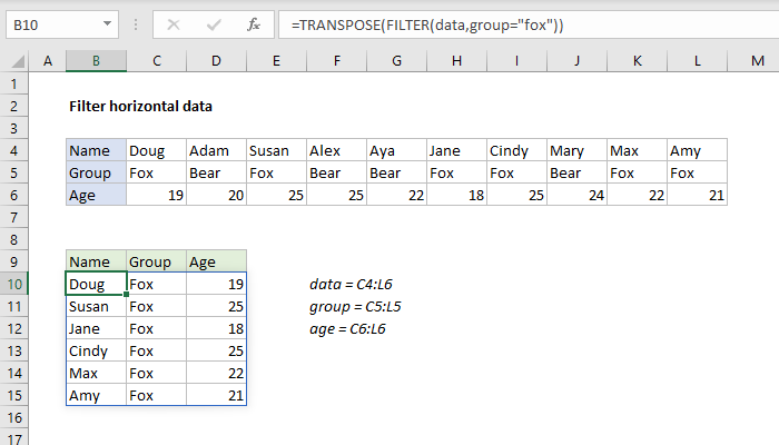
This formula is explained in more detail here .
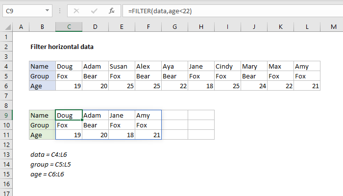
Filter on age
The same basic formula can be used to filter the data in different ways. For example, to filter data to show only columns where age is less than 22, you can use a formula like this:
=FILTER(data,age<22)
FILTER returns the four matching columns of data:
Dynamic Array Formulas are available in Office 365 only.
