Explanation
Note: FILTER is a new dynamic array function in Excel 365 . In other versions of Excel, there are alternatives , but they are more complex.
There are ten columns of data in the range C4:L6. The goal is to filter this horizontal data and extract only columns (records) where the group is “fox”. For convenience and readability, the worksheet contains three named ranges : data (C4:L6) and group (C5:L5), and age (C6:L6).
The FILTER function can be used to extract data arranged vertically (in rows) or horizontally (in columns). FILTER will return the matching data in the same orientation. No special setup is required. In the example shown, the formula in C9 is:
=FILTER(data,group="fox")
Working from the inside out, the include argument for FILTER is a logical expression:
group="fox" // test for "fox"
When the logical expression is evaluated, it returns an array of 10 TRUE and FALSE values:
{TRUE,FALSE,TRUE,FALSE,FALSE,TRUE,TRUE,TRUE,TRUE,FALSE}
Note: the commas (,) in this array indicate columns. Semicolons (;) would indicate rows.
The array contains one value per column in the data, and each TRUE corresponds to a column where the group is “fox”. This array is returned directly to FILTER as the include argument, and it performs the actual filtering:
FILTER(data,{TRUE,FALSE,TRUE,FALSE,FALSE,TRUE,TRUE,TRUE,TRUE,FALSE})
Only data that corresponds to TRUE values passes the filter, so FILTER returns the 6 columns where the group is “fox”. FILTER returns this data in the original horizontal structure. Because FILTER is a dynamic array function , the results spill into the range C9:H11.
This is a dynamic solution – if any source data in C4:L6 changes, the results from FILTER automatically update.
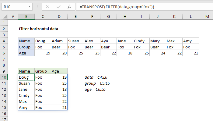
Transpose to vertical format
To transpose the results from FILTER into a vertical (rows) format, you can wrap the TRANSPOSE function around the FILTER function like this:
=TRANSPOSE(FILTER(data,group="fox"))
The result looks like this:
This formula is explained in more detail here .
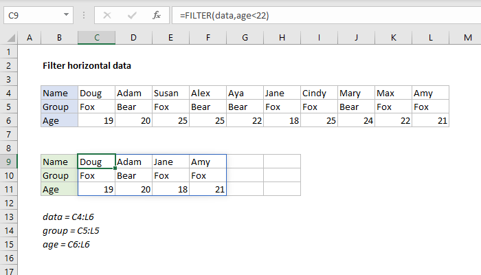
Filter on age
The same basic formula can be used to filter the data in different ways. For example, to filter data to show only columns where age is less than 22, you can use a formula like this:
=FILTER(data,age<22)
FILTER returns the four matching columns of data:
Dynamic Array Formulas are available in Office 365 only.
Explanation
The goal in this example is to display the last 3 valid entries from the table shown, where “valid” is defined as a temperature of less than 75 in the “Temp” column. At a high level, the FILTER function is used to filter entries based on a logical test, and the INDEX function is used to extract the last 3 entries from the filtered list. Working from the inside out, we use the SEQUENCE function to construct a row number value for the INDEX function like this:
SORT(SEQUENCE(3,1,SUM(--(temp<75)),-1))
SEQUENCE is configured to create an array of 3 rows x 1 column. The step value is -1, and the start number is defined by this snippet:
SUM(--(temp<75)) // returns 7
Here we are counting temp values less than 75. Because the named range temp contains twelve values, the result is an array of 12 TRUE and FALSE values:
{TRUE;TRUE;TRUE;FALSE;FALSE;TRUE;TRUE;FALSE;FALSE;TRUE;FALSE;TRUE}
The double negative (–) is used to coerce the TRUE and FALSE results to 1s and 0s, and the SUM function returns the total:
SUM({1;1;1;0;0;1;1;0;0;1;0;1}) // returns 7
This number is returned directly to SEQUENCE for the start value. Now we have:
=SORT(SEQUENCE(3,1,7,-1))
=SORT({7;6;5})
={5;6;7}
We use SORT to ensure that values are returned in the same order they appear in the source data. This array is handed off to the INDEX function as the row_num argument:
=INDEX(FILTER(data,temp<75),{5;6;7},SEQUENCE(1,COLUMNS(data)))
In a similar way, SEQUENCE is also used to generate an array for columns:
SEQUENCE(1,COLUMNS(data)) // returns {1,2,3}
which is given to INDEX for the columns argument. Now we have:
=INDEX(FILTER(data,temp<75),{5;6;7},{1,2,3})
The next step is to construct the array for INDEX to work with. We only want to work with “valid” entries, so we use the FILTER function to retrieve a list of entries where the temp value is less than 75:
FILTER(data,temp<75)
The array argument is data, and the include argument is the expression temp <75. This can be translated literally as “return values from the named range data where values in temp are less than 75”. The result is a 2D array with 3 columns and 7 rows:
{"0100",72,5;"0101",74,8;"0102",74,7;"0105",72,8;"0106",71,6;"0109",74,9;"0111",72,8}
Notice rows associated temp values greater than or equal to 75 have been removed. This array is returned to the INDEX function for its array argument.
Finally, the INDEX function returns the last 3 entries from the array returned by FILTER.
Note: Both the value for n and the logic used to test for valid entries is arbitrary in this example and can be adjusted as needed to suit your needs.
