Explanation
This formula relies on the FILTER function to retrieve data based on a logical test built with the COUNTIF function:
=FILTER(list1,COUNTIF(list2,list1))
working from the inside out, the COUNTIF function is used to create the actual filter:
COUNTIF(list2,list1)
Notice we are using list2 as the range argument, and list1 as the criteria argument. In other words, we are asking COUNTIF to count all values in list1 that appear in list2. Because we are giving COUNTIF multiple values for criteria, we get back an array with multiple results:
{1;1;0;1;0;1;0;0;1;0;1;1}
Note the array contains 12 counts, one for each value in list1 . A zero value indicates a value in list1 that is not found in list2 . Any other positive number indicates a value in list1 that is found in list2 . This array is returned directly to the FILTER function as the include argument:
=FILTER(list1,{1;1;0;1;0;1;0;0;1;0;1;1})
The FILTER function uses the array as a filter. Any value in list1 associated with a zero is removed, while any value associated with a positive number survives.
The result is an array of 7 matching values which spill into the range F5:F11. If data changes, FILTER will recalculate and return a new list of matching values based on the new data.
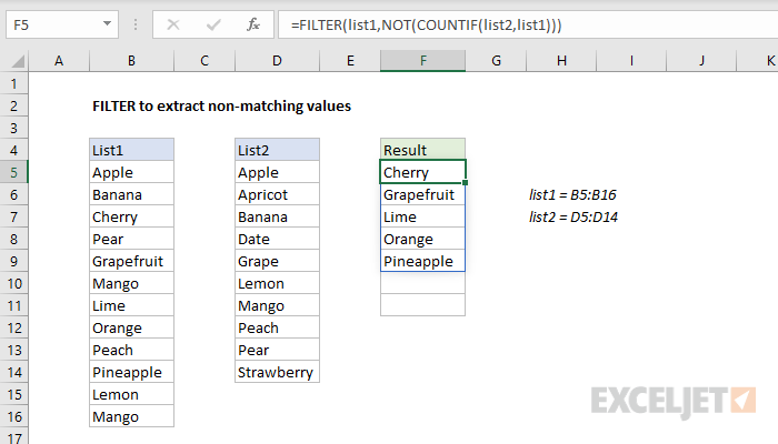
Non-matching values
To extract non-matching values from list1 (i.e. values in list1 that don’t appear in list2 ) you can add the NOT function to the formula like this:
=FILTER(list1,NOT(COUNTIF(list2,list1)))
The NOT function effectively reverses the result from COUNTIF – any non-zero number becomes FALSE, and any zero value becomes TRUE. The result is a list of the values in list1 that are not present in list2 .
With INDEX
It is possible to create a formula to extract matching values without the FILTER function, but the formula is more complex. One option is to use the INDEX function in a formula like this:
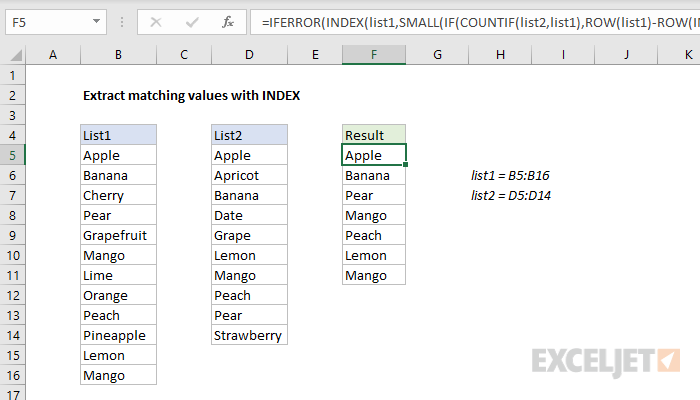
The formula in G5, copied down is:
=IFERROR(INDEX(list1,SMALL(IF(COUNTIF(list2,list1),ROW(list1)-ROW(INDEX(list1,1,1))+1),ROWS($F$5:F5))),"")
Note: this is an array formula and must be entered with control + shift + enter, except in Excel 365 .
The core of this formula is the INDEX function , which receives list1 as the array argument. Most of the remaining formula simply calculates the row number to use for matching values. This expression generates a list of relative row numbers :
ROW(list1)-ROW(INDEX(list1,1,1))+1
which returns an array of 12 numbers representing the rows in list1 :
{1;2;3;4;5;6;7;8;9;10;11;12}
These are filtered with the IF function and the same logic used above in FILTER, based on the COUNTIF function:
COUNTIF(list2,list1) // find matching values
The resulting array looks like this:
{1;2;FALSE;4;FALSE;6;FALSE;FALSE;9;FALSE;11;12} // result from IF
This array is delivered directly to the SMALL function , which is used to fetch the next matching row number as the formula is copied down the column. The k value for SMALL (think nth) is calculated with an expanding range :
ROWS($G$5:G5) // incrementing value for k
The IFERROR function is used to trap errors that occur when the formula is copied down and runs out of matching values. For another example of this idea, see this formula .
Explanation
Although FILTER is more commonly used to filter rows, you can also filter columns, the trick is to supply an array with the same number of columns as the source data. In this example, we construct the array we need with boolean logic , also called Boolean algebra.
In Boolean algebra, multiplication corresponds to AND logic, and addition corresponds to OR logic . In the example shown, we are using Boolean algebra with OR logic (addition) to target only the columns A, C, and E like this:
(B4:G4="a")+(B4:G4="c")+(B4:G4="e")
After each expression is evaluated, we have three arrays of TRUE/FALSE values:
{TRUE,FALSE,FALSE,FALSE,FALSE,FALSE}+
{FALSE,FALSE,TRUE,FALSE,FALSE,FALSE}+
{FALSE,FALSE,FALSE,FALSE,TRUE,FALSE}
The math operation (addition) converts the TRUE and FALSE values to 1s and 0s, so you can think of the operation like this:
{1,0,0,0,0,0}+
{0,0,1,0,0,0}+
{0,0,0,0,1,0}
In the end, we have a single horizontal array of 1s and 0s:
{1,0,1,0,1,0}
which is delivered directly to the FILTER function as the include argument:
=FILTER(B5:G12,{1,0,1,0,1,0})
Notice there are 6 columns in the source data and 6 values in the array, all either 1 or 0. FILTER uses this array as a filter to include only columns 1, 3, and 5 from the source data. Columns 2, 4, and 6 are removed. In other words, the only columns that survive are associated with 1s.
With the MATCH function
Applying OR logic with addition as shown above works fine, but it doesn’t scale well, and makes it impossible to use a range of values from a worksheet as criteria. As an alternative, you can use the MATCH function together with the ISNUMBER function like this to construct the include argument more efficiently:
=FILTER(B5:G12,ISNUMBER(MATCH(B4:G4,{"a","c","e"},0)))
The MATCH function is configured to look for all column headers in the array constant {“a”,“c”,“e”} as shown. We do it this way so that the result from MATCH has dimensions compatible with the source data, which contains 6 columns. Notice also that the third argument in MATCH is set as zero to force an exact match.
After MATCH runs, it returns an array like this:
{1,#N/A,2,#N/A,3,#N/A}
This array goes directly into ISNUMBER, which returns another array:
{TRUE,FALSE,TRUE,FALSE,TRUE,FALSE}
As above, this array is horizontal and contains 6 values separated by commas. FILTER uses the array to remove columns 2, 4, and 6.
With a range
Since the column headers are already on the worksheet in the range I4:K4, the formula above can easily be adapted to use the range directly like this:
=FILTER(B5:G12,ISNUMBER(MATCH(B4:G4,I4:K4,0)))
The range I4:K4 is evaluated as {“a”,“c”,“e”}, and behaves just like the array constant in the formula above.
