Purpose
Return value
Syntax
=FIND(find_text,within_text,[start_num])
- find_text - The substring to find.
- within_text - The text to search within.
- start_num - [optional] The starting position in the text to search. Optional, defaults to 1.
Using the FIND function
The FIND function returns the position (as a number) of one text string inside another. In the most basic case, you can use FIND to locate the position of a substring in a text string. You can also use FIND to check if a cell contains specific text. FIND is case-sensitive, which means it distinguishes between uppercase and lowercase letters. This behavior is automatic and cannot be disabled. Here are a few key points to remember about the FIND function:
- FIND returns the position of one text string inside another as a number .
- When FIND cannot locate the search string, it returns a #VALUE error.
- If the search string appears more than once, FIND returns the first position .
- FIND is case-sensitive and will evaluate “Apple” and “apple” as different text strings.
- FIND does not support wildcards like *?~ when searching for text.
- FIND will return 1 if the search string ( find_text ) is empty.
Note: The SEARCH function is similar to the FIND function. Both functions return the position of one text string inside another. However, unlike FIND, SEARCH is not case-sensitive and does support wildcards.
Basic syntax
The basic syntax of the FIND function looks like this
FIND(find_text,within_text,[start_num])
- find_text : The text you want to find (the search string). This is a substring that Excel searches for within another text string. The text must be entered in double quotes if you are hardcoding the value into the formula. Otherwise, you can refer to a cell that contains the text.
- within_text : The text string that contains the text you want to find. Often this is a cell reference that contains the text, but you can also hardcode a text string in double quotes.
- start_num (optional): The character at which to begin searching, as a numeric position. The first character in within_text is considered position 1. If omitted, the search starts at the beginning of the within_text .
Basic example
The FIND function is designed to look inside a text string for a specific substring. When FIND locates the substring, it returns the position of the substring in the text as a number. If the substring is not found, FIND returns a #VALUE error. For example:
=FIND("p","apple") // returns 2
=FIND("z","apple") // returns #VALUE!
=FIND("apple","Pineapple") // returns 5
Note that text values entered directly into FIND must be enclosed in double quotes (""). As mentioned above, the FIND function is always case-sensitive:
=FIND("a","Apple") // returns #VALUE!
=FIND("A","Apple") // returns 1
=FIND("Apple","Pineapple") // returns #VALUE!
The worksheet below shows the same examples translated into formulas based on cell references:

Forcing a TRUE or FALSE result
By default, the FIND function returns a number when a search string is found and a #VALUE! error when not. This is inconvenient in cases where you simply want to know if the search string has been found or not. To force a TRUE or FALSE result, you can nest the FIND function inside the ISNUMBER function . ISNUMBER returns TRUE for numeric values and FALSE for anything else. If FIND locates the substring, it returns the position as a number, and ISNUMBER returns TRUE:
=ISNUMBER(FIND("p","apple")) // returns TRUE
=ISNUMBER(FIND("z","apple")) // returns FALSE
If FIND doesn’t locate the substring, it returns an error, and ISNUMBER returns FALSE. You can replace the FIND function above with the SEARCH function if you need support for wildcards. For a more detailed explanation of this approach, with many more examples, see this example .
If cell contains
Once you have a TRUE or FALSE result, you can combine the FIND function with the IF function to create “if cell contains” logic. The generic pattern for this formula looks like this:
=IF(ISNUMBER(FIND(substring,A1)), "Yes", "No")
Instead of returning TRUE or FALSE, the formula above will return “Yes” if the substring is found and “No” if not. You can use the same idea to mark or “flag” items of interest. For example, in the worksheet below, we are using a FIND with IF to flag email addresses that contain “abc” with an “x”.
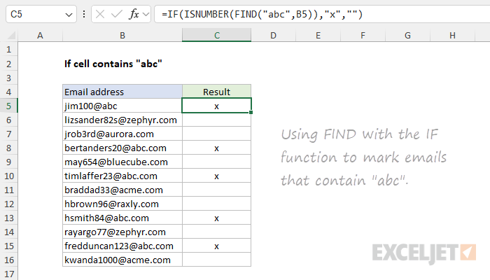
The formula in C5, copied down, is:
=IF(ISNUMBER(FIND("abc",B5)),"x","")
Start number
The FIND function has an optional argument called start_num , that controls where FIND should begin looking for a substring. To find the first match of “the” in any combination of upper or lowercase, you can omit start_num , which defaults to 1:
=FIND("x","20 x 30 x 50") // returns 4
FIND returns 4 since the first “x” appears at position 4. To find the second “x”, enter 5 for start_num :
=FIND("x","20 x 30 x 50",5) // returns 9
In this case, FIND returns 9 since it starts searching after the first “x”. You can effectively find the second “x” in cell A1 in a single formula by using FIND twice like this:
=FIND(A1,FIND("x",A1)+1)
The inner FIND returns the location of the first “x”. We then add 1 and the result is used as the start_num in the outer FIND. The result is the location of the second “x” in cell A1.
Wildcards
The FIND function does not support wildcards. See the SEARCH function .
More advanced formulas
The FIND function shows up in many more advanced formulas that work with text. FIND is interchangeable with SEARCH, so you will often see SEARCH substituted for FIND (and vice versa) depending on the need for case sensitivity and wildcard support. Here are a few examples:
- Cell contains one of many things - tests a cell for more than one text string simultaneously.
- Sum if cells contain either x or y - sum numbers when associated cells contain one value or another value
- Filter if text contains - extract values from a set of data with “contains-type” logic
- Categorize text with keywords - return an appropriate category based on if a cell contains one of several text values.
- Filter based on partial match - extract records from an Excel Table based on a partial match.
Notes
- The FIND function returns the location of the first find_text in within_text .
- The location is returned as the number of characters from the start.
- Start_num is optional and defaults to 1.
- FIND returns 1 when find_text is empty.
- FIND returns #VALUE if find_text is not found.
- FIND is case-sensitive but does not support wildcards.
- Use the SEARCH function to find a substring with wildcards.
Purpose
Return value
Syntax
=FIXED(number,[decimals],[no_commas])
- number - The number to round and format.
- decimals - [optional] Number of decimals to use. Default is 2.
- no_commas - [optional] Suppress commas. TRUE = no commas, FALSE = commas. Default is FALSE.
Using the FIXED function
The FIXED function converts a number to text, rounding to a given number of decimals. Like the Number format available on the home tab of the ribbon, the FIXED function will round the number as needed using the given number of decimal places. The main difference between applying a number format and using FIXED is that the FIXED function converts the number to text, whereas a number format just changes the way a number is displayed.
The FIXED function takes three arguments , number , decimals , and no_commas . Number is the number to convert. Decimals is the number of digits to which number will be rounded on the right of the decimal point. If decimals is negative, number will be rounded to the left of the decimal point. Decimals is optional and defaults to 2.
The no_commas argument is a Boolean that controls whether commas will be added to the result. No_commas is optional and defaults to FALSE. To prevent commas, set no_commas to TRUE.
Note: the FIXED function returns text and not a number, so the result cannot be used in a numeric calculation. If the goal is to format a number and retain its numeric property, applying a standard number format is a better option. Video: How to use number formatting .
Examples
In the example shown above, the formula in E5, copied down, is:
=FIXED(B5,C5,D5)
At each new row, FIXED returns a result based on the number in column B, the decimals in column C, and comma setting in column D.
Number is the only required argument. By default, FIXED will round to 2 decimal places and insert commas for thousands:
=FIXED(1000) // returns "1,000.00"
=FIXED(1000,0) // returns "1,000"
=FIXED(1000,0,FALSE) // returns "1000"
The FIXED function can be useful when you want to concatenate a number with other text. The example below shows how the output from the PI function can be trimmed by FIXED:
="PI is about "&PI() // returns "PI is about 3.14159265358979"
="PI is about "&FIXED(PI()) // returns "PI is about 3.14"
FIXED vs. TEXT
The FIXED function is a specialized function to apply Number formatting only. The TEXT function is a generalized function that does the same thing in a more flexible way. TEXT can convert numeric values to many different number formats , including currency, date, time, percentage, and so on.
Notes
- The output from FIXED is text. To simply format a number, apply a number format instead.
- The FIXED function converts a number to text using a number format like: 0.00 or #,##0
- The default for decimals is 2. If decimals is negative, number will be rounded to the left of the decimal point.
- The TEXT function is a more flexible way to achieve the same result.
