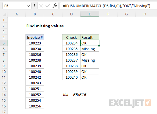
Explanation
The goal is to identify invoice numbers in range D5:D11 that are missing in range B5:B16 (named list ). Two good ways to solve this problem in Excel are the COUNTIF function and the MATCH function . Both approaches are explained below.
COUNTIF function
COUNTIF counts cells in a range that meet a given condition (criteria). If no cells meet the criteria, COUNTIF returns zero. The generic syntax for COUNTIF is:
=COUNTIF(range,criteria)
To check for missing invoices, combine COUNTIF with the IF function . The formula in G5 is:
=IF(COUNTIF(list,D5),"OK","Missing")
Notice the COUNTIF formula appears inside the IF function as the logical_test argument. Normally, the IF function requires a logical test to return TRUE or FALSE. However, Excel will automatically evaluate any non-zero number as TRUE and the number zero (0) as FALSE. As the formula is copied down column E, COUNTIF returns the count of each invoice in column D in the named range list (B5:B16). When the count is non-zero, The IF function returns “OK”. If the invoice is not found in list , COUNTIF returns zero (0), which evaluates as FALSE, and IF returns “Missing”.
Alternative with MATCH
Another approach is to use the MATCH function . MATCH locates the position of a value in a row, column, or table. The generic syntax for MATCH in exact match mode is:
=MATCH(value,array,0)
The last value, match_type, is set to zero for an exact match. When MATCH finds the lookup value, it returns the position of that value in the array as a number . If MATCH doesn’t find the lookup value, it returns an #N/A error. Use this behavior to build a formula that returns “Missing” or “OK” by testing the result of MATCH with the ISNUMBER function :
=IF(ISNUMBER(MATCH(D5,list,0)),"OK","Missing")
As the formula is copied down column E, MATCH returns the position of each invoice in column D in the named range list (B5:B16). When an invoice number is not found, MATCH returns #N/A. The ISNUMBER function returns TRUE or FALSE, depending on the result from MATCH. The result from ISNUMBER is returned to the IF function as the logical_test , and IF then returns “OK” when an invoice is found and “Missing” when an invoice is not found. The screen below shows this formula in use:

Summary
Explanation
There are certain functions in Excel that return a cell reference as a result rather than a value. Two of these functions are XLOOKUP and INDEX . The presence of the cell reference in the result is not obvious, because Excel immediately resolves the reference to the value in that cell. You can check the reference returned by XLOOKUP or INDEX with the CELL function . This can be useful when debugging a lookup formula to confirm the result being returned.
XLOOKUP function
XLOOKUP is a function in Excel that returns a cell reference as a result instead of a value. You can inspect the reference returned by XLOOKUP by wrapping the formula in the CELL function with “address” as info_type . In the example shown, the formula in cell F6 is:
=CELL("address",XLOOKUP(F4,B5:B17,C5:C17))
Working from the inside out, the formula is an ordinary XLOOKUP formula:
=XLOOKUP(F4,B5:B17,C5:C17)
With a lookup value of “Sat” in cell F4, XLOOKUP returns 325, the Sales amount on the first entry for Saturday. However, underneath the surface, XLOOKUP is actually returning a reference to cell C10. We can check that result by nesting the XLOOKUP function inside the CELL function, and providing “address” for the info_type argument:
=CELL("address",XLOOKUP(F4,B5:B17,C5:C17)) // returns $C$10
The CELL function returns $C$10, the address of the cell returned by XLOOKUP. Note that if we configure XLOOKUP to perform a reverse search, by providing -1 for the search_mode argument, the result is $C$17:
=CELL("address",XLOOKUP(F4,B5:B17,C5:C17,,,-1)) // returns $C$17
This is the address of the second (and last) entry for Saturday in the data.
INDEX and MATCH
Like the XLOOKUP function, the INDEX function is another function that returns an address. The equivalent INDEX and MATCH formula that retrieves the Sales amount for “Sat” in F4 is:
=INDEX(C5:C17,MATCH(F4,B5:B17,0))
By wrapping the formula in the CELL function , we can get Excel to show us the address to the cell returned by INDEX:
=CELL("address",INDEX(C5:C17,MATCH(F4,B5:B17,0))) // returns $C$10
The CELL function returns $C$10, the address of the cell returned by INDEX.