Purpose
Return value
Syntax
=FIXED(number,[decimals],[no_commas])
- number - The number to round and format.
- decimals - [optional] Number of decimals to use. Default is 2.
- no_commas - [optional] Suppress commas. TRUE = no commas, FALSE = commas. Default is FALSE.
Using the FIXED function
The FIXED function converts a number to text, rounding to a given number of decimals. Like the Number format available on the home tab of the ribbon, the FIXED function will round the number as needed using the given number of decimal places. The main difference between applying a number format and using FIXED is that the FIXED function converts the number to text, whereas a number format just changes the way a number is displayed.
The FIXED function takes three arguments , number , decimals , and no_commas . Number is the number to convert. Decimals is the number of digits to which number will be rounded on the right of the decimal point. If decimals is negative, number will be rounded to the left of the decimal point. Decimals is optional and defaults to 2.
The no_commas argument is a Boolean that controls whether commas will be added to the result. No_commas is optional and defaults to FALSE. To prevent commas, set no_commas to TRUE.
Note: the FIXED function returns text and not a number, so the result cannot be used in a numeric calculation. If the goal is to format a number and retain its numeric property, applying a standard number format is a better option. Video: How to use number formatting .
Examples
In the example shown above, the formula in E5, copied down, is:
=FIXED(B5,C5,D5)
At each new row, FIXED returns a result based on the number in column B, the decimals in column C, and comma setting in column D.
Number is the only required argument. By default, FIXED will round to 2 decimal places and insert commas for thousands:
=FIXED(1000) // returns "1,000.00"
=FIXED(1000,0) // returns "1,000"
=FIXED(1000,0,FALSE) // returns "1000"
The FIXED function can be useful when you want to concatenate a number with other text. The example below shows how the output from the PI function can be trimmed by FIXED:
="PI is about "&PI() // returns "PI is about 3.14159265358979"
="PI is about "&FIXED(PI()) // returns "PI is about 3.14"
FIXED vs. TEXT
The FIXED function is a specialized function to apply Number formatting only. The TEXT function is a generalized function that does the same thing in a more flexible way. TEXT can convert numeric values to many different number formats , including currency, date, time, percentage, and so on.
Notes
- The output from FIXED is text. To simply format a number, apply a number format instead.
- The FIXED function converts a number to text using a number format like: 0.00 or #,##0
- The default for decimals is 2. If decimals is negative, number will be rounded to the left of the decimal point.
- The TEXT function is a more flexible way to achieve the same result.
Purpose
Return value
Syntax
=LEFT(text,[num_chars])
- text - The text from which to extract characters.
- num_chars - [optional] The number of characters to extract, starting on the left. Default = 1.
Using the LEFT function
The LEFT function extracts a given number of characters from the left side of a supplied text string. The first argument, text , is the text string to extract from. This is typically a reference to a cell that contains text. The second argument, called num_chars , specifies the number of characters to extract. If num_chars is not provided, it defaults to 1. If num_chars is greater than the number of characters available, LEFT returns the entire text string. Although LEFT is a simple function, it shows up in many more advanced formulas that test or manipulate text in a specific way.
LEFT function basics
To extract text with LEFT, just provide the text and the number of characters to extract. The formulas below show how to extract one, two, and three characters with LEFT:
=LEFT("apple",1) // returns "a"
=LEFT("apple",2) // returns "ap"
=LEFT("apple",3) // returns "app"
If the optional argument num_chars is not provided, it defaults to 1:
=LEFT("ABC") // returns "A"
If num_chars exceeds the length of the text string, LEFT returns the entire string:
=LEFT("apple",100) // returns "apple"
When LEFT is used on a numeric value, the result is text:
=LEFT(1000,3) // returns "100" as text
Example - abbreviate month names
The LEFT function can be used to abbreviate text values. For example, to extract the first three characters of “January” you can use LEFT like this:
=LEFT("January",3) // returns "Jan"
Of course, it doesn’t make sense to abbreviate a text string that you have to type into a formula. A more typical example is to abbreviate text values that already exist in cells , as seen in the worksheet below. The formula in cell D5, copied down, is:
=LEFT(B5,3)

Notice num_chars is provided as 3 to extract the first 3 letters of each month.
Example - extract the first character
An interesting quirk of the LEFT function is that the number of characters to extract is not required and defaults to 1. This can be useful in cases where you only want to extract the first character of a text string, as seen below. Here, the formula in cell D5 looks like this:
=LEFT(B5)

As you can see, without a value for num_chars , LEFT extracts the first letter of each month.
Example - LEFT with UPPER
You can easily combine LEFT with other functions in Excel to get a more specific result. For example, you could nest the LEFT function inside the UPPER function to convert the result from LEFT to uppercase. You can see this approach in the worksheet below, where the formula in cell D5 looks like this:
=UPPER(LEFT(B5,3))

Example - LEFT with IF
You can easily combine the LEFT function with the IF function to create “if cell begins with” logic. In the example below, a formula is used to flag codes that begin with “xyz” with an “x”. The formula in cell D5 is:
=IF(LEFT(B5,3)="xyz","x","")
<img loading=“lazy” src=“https://exceljet.net/sites/default/files/styles/original_with_watermark/public/images/functions/inline/left_function_example_if_cell_begins_with.png" onerror=“this.onerror=null;this.src=‘https://blogger.googleusercontent.com/img/a/AVvXsEhe7F7TRXHtjiKvHb5vS7DmnxvpHiDyoYyYvm1nHB3Qp2_w3BnM6A2eq4v7FYxCC9bfZt3a9vIMtAYEKUiaDQbHMg-ViyGmRIj39MLp0bGFfgfYw1Dc9q_H-T0wiTm3l0Uq42dETrN9eC8aGJ9_IORZsxST1AcLR7np1koOfcc7tnHa4S8Mwz_xD9d0=s16000';" alt=” LEFT function example - if cell begins with “xyz” - 4”>
As the formula is copied down, the LEFT function returns the first 3 characters in each value, which are compared to “xyz” as a logical test. When the result is TRUE, IF returns “x”. When the result is FALSE, IF returns an empty string “”. The result is that the codes in column B that begin with “xyz” are clearly marked.
LEFT is not case-sensitive as you can see in the formula above. To perform a case-sensitive test you can combine LEFT with the EXACT function. Example here .
Example - LEFT with FIND
A common challenge with the LEFT function is extracting a variable number of characters, depending on the location of a specific character in the text string. To handle this situation you can use the LEFT function together with the FIND function in a generic formula like this:
=LEFT(text,FIND(character,text)-1) // extract text up to character
FIND returns the position of the character, and LEFT returns all text to the left of that position. The screen below shows how this formula can be applied in a worksheet. The formula in cell D5 is:
=LEFT(B5,FIND(" ",B5)-1)
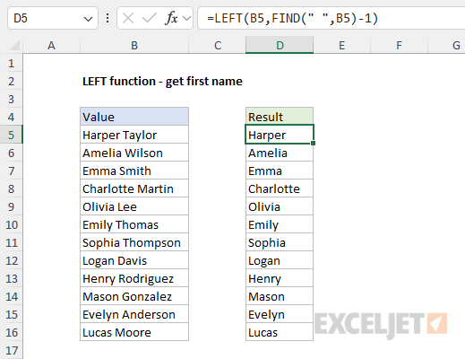
As the formula is copied down, the FIND function returns the position of the space character " " as a number. The result, minus one, is returned to the LEFT function as the num_chars argument, which then extracts all text up to the first space. You can read a more detailed explanation here .
Related functions
The LEFT function is used to extract text from the left side of a text string. Use the RIGHT function to extract text starting from the right side of the text, and the MID function to extract from the middle of text. The LEN function returns the length of a text string as a count of characters and is often combined with LEFT, MID, and RIGHT.
In the latest version of Excel, newer functions like TEXTBEFORE , TEXTAFTER , and TEXTSPLIT greatly simplify certain text operations and make some traditional formulas that use the LEFT function obsolete. Example here .
Notes
- LEFT is not case-sensitive.
- LEFT can extract numbers as well as text.
- The output from LEFT is always text.
- LEFT ignores number formatting when extracting characters.
- Num_chars is optional and defaults to 1.
