Explanation
The core of this formula is the MOD function. MOD takes a number and divisor, and returns the remainder after division, which makes it useful for formulas that need to do something every nth time.
In this case, the number is created with the COLUMN function, which return the column number of cell B8, the number 2, minus 1, which is supplied as an “offset”. We use an offset, because we want to make sure we start counting at 1, regardless of the actual column number.
The divisor is hardcoded as 3, since we want to do something every 3rd month. By testing for a zero remainder, this expression will return TRUE at the 3rd, 6th, 9th, and 12th months:
MOD(COLUMN(B8)-1,3)=0
Finally, IF simply evaluates the MOD expression and returns value in B5 (coded as an absolute reference to prevent changes as the formula is copied) when TRUE and zero when FALSE.
Working with a date
If you need to repeat a value every n months, and you are working directly with dates, see this example .
Explanation
At the core, this formula is composed of two sets of the COUNTIF function wrapped in the IF function . The outer IF + COUNTIF first checks to see if the value in question (B4) appears more than once in the list:
=IF(COUNTIF($B$4:$B$11,B4)>1
If not, the outer IF function returns an empty string ("") as a final result. If the value does appear more than once, we run another IF + COUNTIF combo. This one does the work of flagging duplicates:
IF(COUNTIF($B$4:B4,B4)=1,"x","xx")
This part of the formula uses an expanding reference ($B$4:B4) that expands as the formula is copied down the column. The first B4 in the range is absolute (locked), and the second is relative, so it changes as the formula is copied down the list.
Remember that this part of the formula is only executed if the first COUNTIF returns a number greater than 1. So, at each row, the formula checks the count inside the range up to the current row. If the count is 1, we mark the duplicate with “x”, since it’s the first one we’ve seen. If it’s not 1, we know it must be a subsequent duplicate, and we mark it with “xx”
Basic formula
To flag the first duplicate in a list only with a 0 or 1, you can use this stripped-down formula, which uses an expanding range and the COUNTIFS function .
=(COUNTIFS($B$5:B5,B5)=2)+0
This formula will return 1 only when a value has been encountered twice – the first occurrence will return zero:
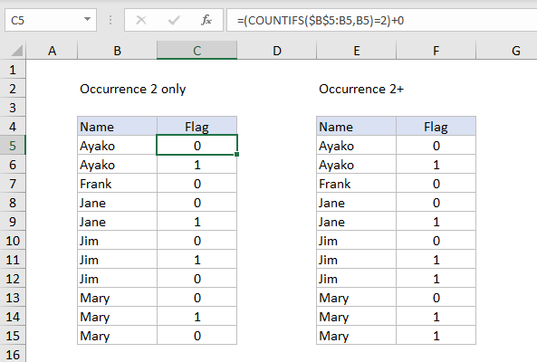
To flag the second and all subsequent occurrences, the formula in F5 above is:
=(COUNTIFS($E$5:E5,E5)>=2)+0
Note: In both examples, adding zero is just a simple way to coerce TRUE and FALSE values to 1 and 0.
Also, using COUNTIFS instead of COUNTIF makes it possible to evaluate values in other columns as part of the test for duplicates. Each additional column also needs to be entered as an expanding range.
